With mortgage rates at a historical low there are inklings the US housing market is heating up again. Buying a home is a huge decision and in a perfect world everyone weighs their options and makes a (relatively) rational choice.
One approach is to lay out all the mortgage offers and compare how much more we’re paying over the life of the loan. In this article I want to achieve a few things:
- Create a loan amortization table
- Visualize and compare the different scenarios
- Develop everything in python
Load modules
import pandas as pd
import numpy as np
import numpy_financial as npf #DOWNLOAD: pip3 install numpy-financial
import matplotlib.pyplot as plt
import seaborn as sns

sns.set(style="darkgrid")
Define function
To build our amortization schedule we can write a python function to accept three arguments: interest rate, mortgage amount, and loan duration.
def amortization_schedule(input_intrate, mortgage, years):

  ##### PARAMETERS #####
  # CONVERT MORTGAGE AMOUNT TO NEGATIVE BECAUSE MONEY IS GOING OUT
  mortgage_amount = -(mortgage)
  interest_rate = (input_intrate / 100) / 12
  periods = years*12
  # CREATE ARRAY
  n_periods = np.arange(years * 12) + 1

  ##### BUILD AMORTIZATION SCHEDULE #####
  # INTEREST PAYMENT
  interest_monthly = npf.ipmt(interest_rate, n_periods, periods, mortgage_amount)

  # PRINCIPAL PAYMENT
  principal_monthly = npf.ppmt(interest_rate, n_periods, periods, mortgage_amount)

  # JOIN DATA
  df_initialize = list(zip(n_periods, interest_monthly, principal_monthly))
  df = pd.DataFrame(df_initialize, columns=['period','interest','principal'])

  # MONTHLY MORTGAGE PAYMENT
  df['monthly_payment'] = df['interest'] + df['principal']

  # CALCULATE CUMULATIVE SUM OF MORTAGE PAYMENTS
  df['outstanding_balance'] = df['monthly_payment'].cumsum()

  # REVERSE VALUES SINCE WE ARE PAYING DOWN THE BALANCE
  df.outstanding_balance = df.outstanding_balance.values[::-1]

  return(df)
Build scenarios
Let’s assume a $500k loan for a standard length of 30 years with a few varying interest rates.
input_loan = 5e5
input_years = 30

scenario1 = amortization_schedule(4.00, input_loan, input_years)
scenario2 = amortization_schedule(3.00, input_loan, input_years)
scenario3 = amortization_schedule(2.00, input_loan, input_years)
Visualize
plt.figure(figsize=(15,10))

sns.lineplot(x='period', y='outstanding_balance', data=scenario1, color='steelblue');
sns.lineplot(x='period', y='outstanding_balance', data=scenario2, color='salmon');
sns.lineplot(x='period', y='outstanding_balance', data=scenario3, color='seagreen');
plt.axhline(y=5e5, linestyle=':', color='grey')

plt.xlabel("Period")
plt.ylabel("Outstanding Balance ($)")
plt.subplots_adjust(top = 0.94)
plt.suptitle("$500K mortgage over 30 years", x=0.12, horizontalalignment="left", fontsize=15)
plt.figtext(0.9, 0.04, "by: @eeysirhc", horizontalalignment="right")
plt.legend(labels=['4% Interest Rate', '3% Interest Rate', '2% Interest Rate'])

plt.show()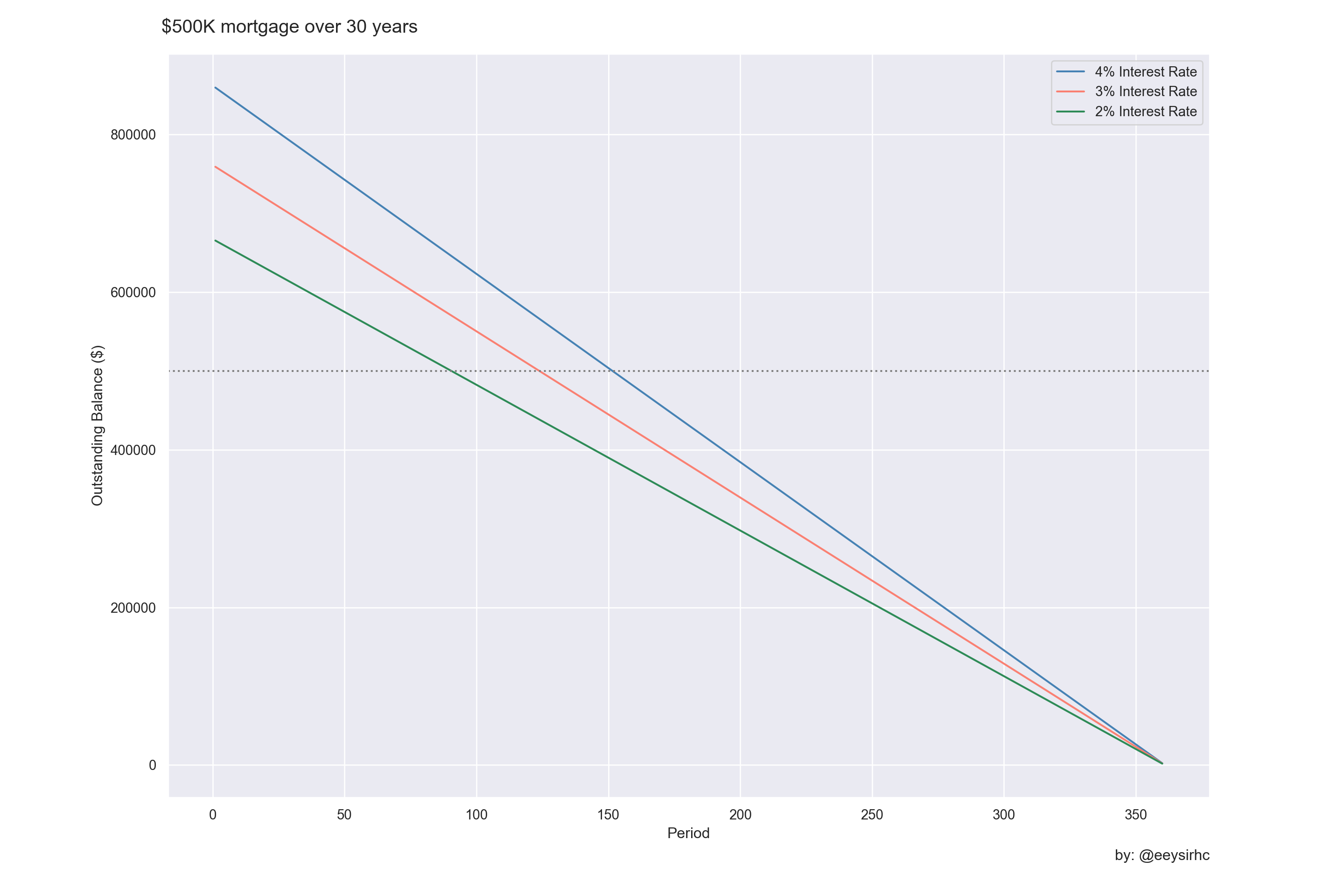
The great thing about this plot is how quickly we can identify the contrast between our different loan offers.
Reviewing the first scenario with 4% interest rate reveals we are paying almost +72% over the life of the entire loan, or an extra $359K in interest.
scenario1[:1]['outstanding_balance'] - input_loan## 0 359347.531838
## Name: outstanding_balance, dtype: float64In fact, for this option the original loan amount doesn’t start paying down until ~13 years later:
scenario1[scenario1['outstanding_balance'] < input_loan][:1]## period interest principal monthly_payment outstanding_balance
## 151 152 1196.352798 1190.72368 2387.076477 498898.983761For comparison the 2% interest rate scenario occurs by year ~8:
scenario3[scenario3['outstanding_balance'] < input_loan][:1]## period interest principal monthly_payment outstanding_balance
## 90 91 669.256966 1178.840398 1848.097363 498986.28813Wrapping up
With a little help from the python programming language we were able to build our own amortization schedule, visualize the remaining balance during the life of the loan, and quickly compare & contrast an assortment of mortgage options.
If you found this useful or interesting then please do not hesitate to share with others on your favorite social media platform!