The US has a peculiar relationship with guns where we frequently observe nontrivial spikes in firearm sales. These are triggered (pun intended) by various political, economic, and social events at the time.
With 2020 being an especially chaotic year, I wanted to explore how that phenomenon is reflected in American gun purchases thus far.
Load modules
import pandas as pd
import matplotlib.pyplot as plt
import seaborn as sns
Retrieve data
I was unable to find confirmed and accurate gun purchase data that is free on the web. However, we can use data from the FBI’s National Instant Criminal Background Check System (NICS) as a proxy.
Note #1: the assumption we are making here is most background checks will result in the sale of a firearm.
The NICS data is stored in PDF format but thanks to the BuzzFeed News team they already wrote the code to parse and sanitize these files. What is even more amazing is how they went the extra mile to update these statistics on a regular basis.
nics_raw = pd.read_csv("https://raw.githubusercontent.com/BuzzFeedNews/nics-firearm-background-checks/master/data/nics-firearm-background-checks.csv")

nics = nics_raw

nics.month = pd.to_datetime(nics.month, infer_datetime_format=True)
Let’s verify what variables are at our disposal:
nics_raw.dtypes## month datetime64[ns]
## state object
## permit float64
## permit_recheck float64
## handgun float64
## long_gun float64
## other float64
## multiple int64
## admin float64
## prepawn_handgun float64
## prepawn_long_gun float64
## prepawn_other float64
## redemption_handgun float64
## redemption_long_gun float64
## redemption_other float64
## returned_handgun float64
## returned_long_gun float64
## returned_other float64
## rentals_handgun float64
## rentals_long_gun float64
## private_sale_handgun float64
## private_sale_long_gun float64
## private_sale_other float64
## return_to_seller_handgun float64
## return_to_seller_long_gun float64
## return_to_seller_other float64
## totals int64
## dtype: objectWith this many variables our analysis can go a million different ways. We’ll limit our scope to a few dimensions and keep them in mind for a future article.
What is the trend in firearm background checks?
nics_total = nics[['month', 'totals']]
nics_total = nics_total.groupby('month').agg('sum').reset_index()

plt.figure(figsize=(15, 10))

sns.lineplot(x='month', y='totals', data=nics_total, marker='o', color='seagreen')
plt.title("Total NICS Firearm Background Checks")
plt.xlabel("")
plt.ylabel("")
plt.figtext(0.9, 0.05, "by: @eeysirhc", horizontalalignment="right")
plt.figtext(0.9, 0.03, "source: Federal Bureau of Investigation", horizontalalignment="right")

plt.show()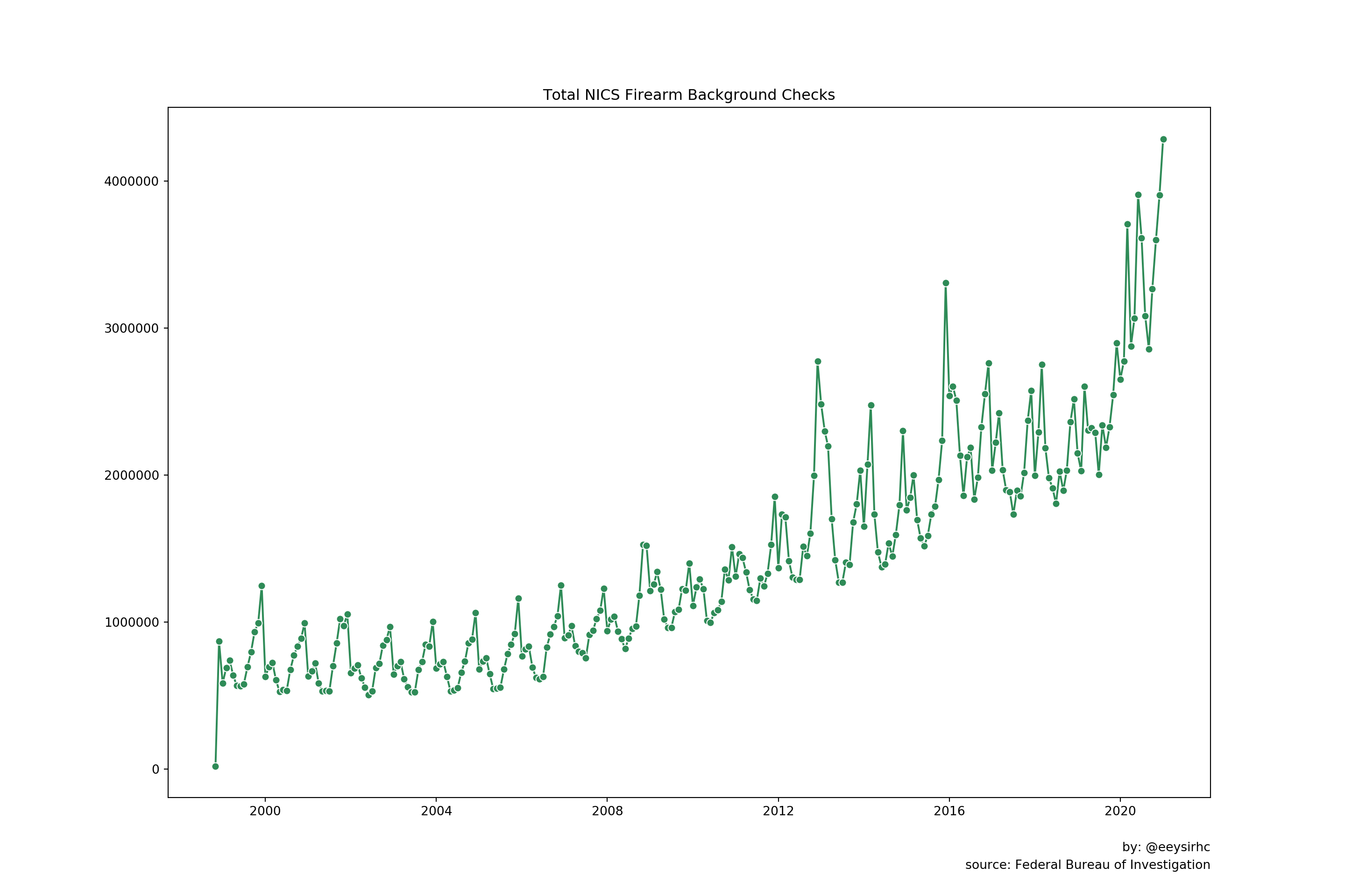
It is quite apparent the 2000s have a steady flow of background checks but that gradually increased over time from 2008 onward. My mind immediately recalls a few major events during those time frames:
- 2000 to 2008 - the Bush administration and the country as a whole was focused on a post-9/11 world with two foreign wars in the Middle East
- 2008 to 2016 - mass shootings plagued the country with the Obama administration attempting to drive domestic policy related to gun control
- 2016 to present - background checks are fairly stable throughout the Trump administration but there is a significant jump in 2020
What type of gun receives the most background checks?
nics_guntype = nics[['month', 'handgun', 'long_gun']]
nics_guntype = nics_guntype.groupby('month').agg('sum').reset_index()

nics_guntype_parsed = (pd.melt(nics_guntype, id_vars=['month'],
    value_vars=['handgun', 'long_gun'], var_name='type'))

plt.figure(figsize=(15, 10))

sns.lineplot(x='month', y='value', hue='type', data=nics_guntype_parsed, marker='o')
plt.title("Total NICS Firearm Background Checks by Type")
plt.xlabel("")
plt.ylabel("")
plt.figtext(0.9, 0.05, "by: @eeysirhc", horizontalalignment="right")
plt.figtext(0.9, 0.03, "source: Federal Bureau of Investigation", horizontalalignment="right")

plt.show()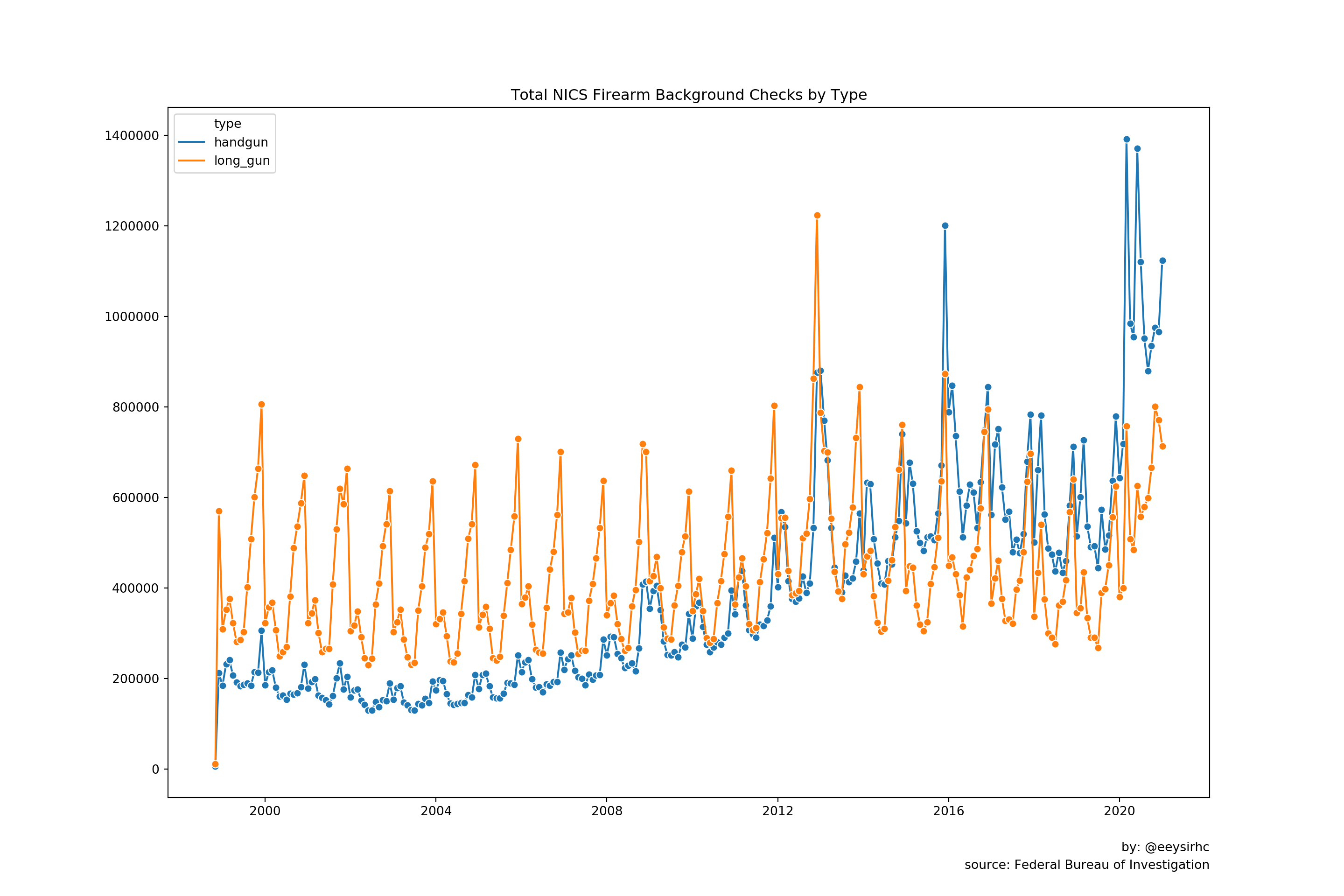
According to this chart, it appears long guns have remained relatively stable for the past two decades. In contrast, we observe an increase in handgun purchases from 2008, surpassing long guns by 2015, and exhibiting a surge in early 2020.
What is the ratio of handgun to long guns?
To better compare the two types of guns we can normalize our values as a ratio: how many handguns are purchased for each long gun (and vice versa)?
nics_ratio = nics_guntype
nics_ratio['handgun_ratio'] = nics_guntype['handgun'] / nics_guntype['long_gun']
nics_ratio['longgun_ratio'] = nics_guntype['long_gun'] / nics_guntype['handgun']

nics_ratio = (pd.melt(nics_ratio, id_vars=['month'],
    value_vars=['handgun_ratio', 'longgun_ratio'], var_name='type'))

plt.figure(figsize=(15, 10))

sns.lineplot(x='month', y='value', hue='type', data=nics_ratio, marker='o')
plt.title("NICS Firearm Background Checks by Ratio of Firearm Type")
plt.xlabel("")
plt.ylabel("")
plt.figtext(0.9, 0.05, "by: @eeysirhc", horizontalalignment="right")
plt.figtext(0.9, 0.03, "source: Federal Bureau of Investigation", horizontalalignment="right")
plt.legend()

plt.show()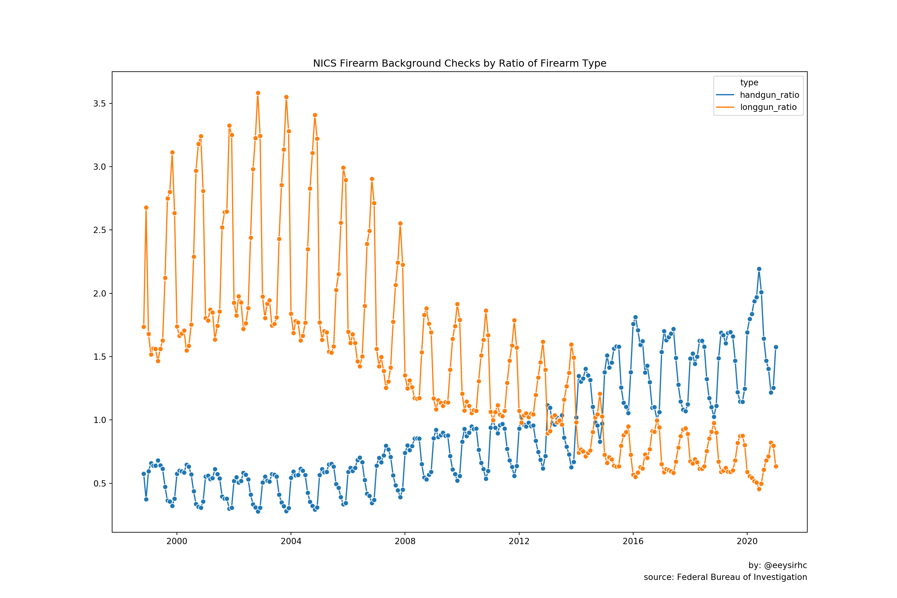
This is quite interesting: even though total long gun background checks have remained flat, the ratio has fallen dramatically.
Indeed, just 20 years ago Americans were purchasing 4-6 long guns for every handgun. By 2020 this trend has flipped where we get about 4 handguns for every long gun!
What caused the influx of gun sales in 2020?
nics_thisyear = nics_guntype_parsed[nics_guntype_parsed['month'] >= '2019-01-01']

plt.figure(figsize=(15, 10))

sns.lineplot(x='month', y='value', hue='type', data=nics_thisyear, marker='o');
plt.title("NICS Firearm Background Checks by Type since 2019")
plt.axvline(x="2020-03-01", color="grey", linestyle='dashed')
plt.axvline(x="2020-06-01", color="grey", linestyle='dashed')
plt.xlabel("")
plt.ylabel("")
plt.ylim(bottom=0, top=2e6);
plt.figtext(0.9, 0.05, "by: @eeysirhc", horizontalalignment="right")
plt.figtext(0.9, 0.03, "source: Federal Bureau of Investigation", horizontalalignment="right")

plt.show()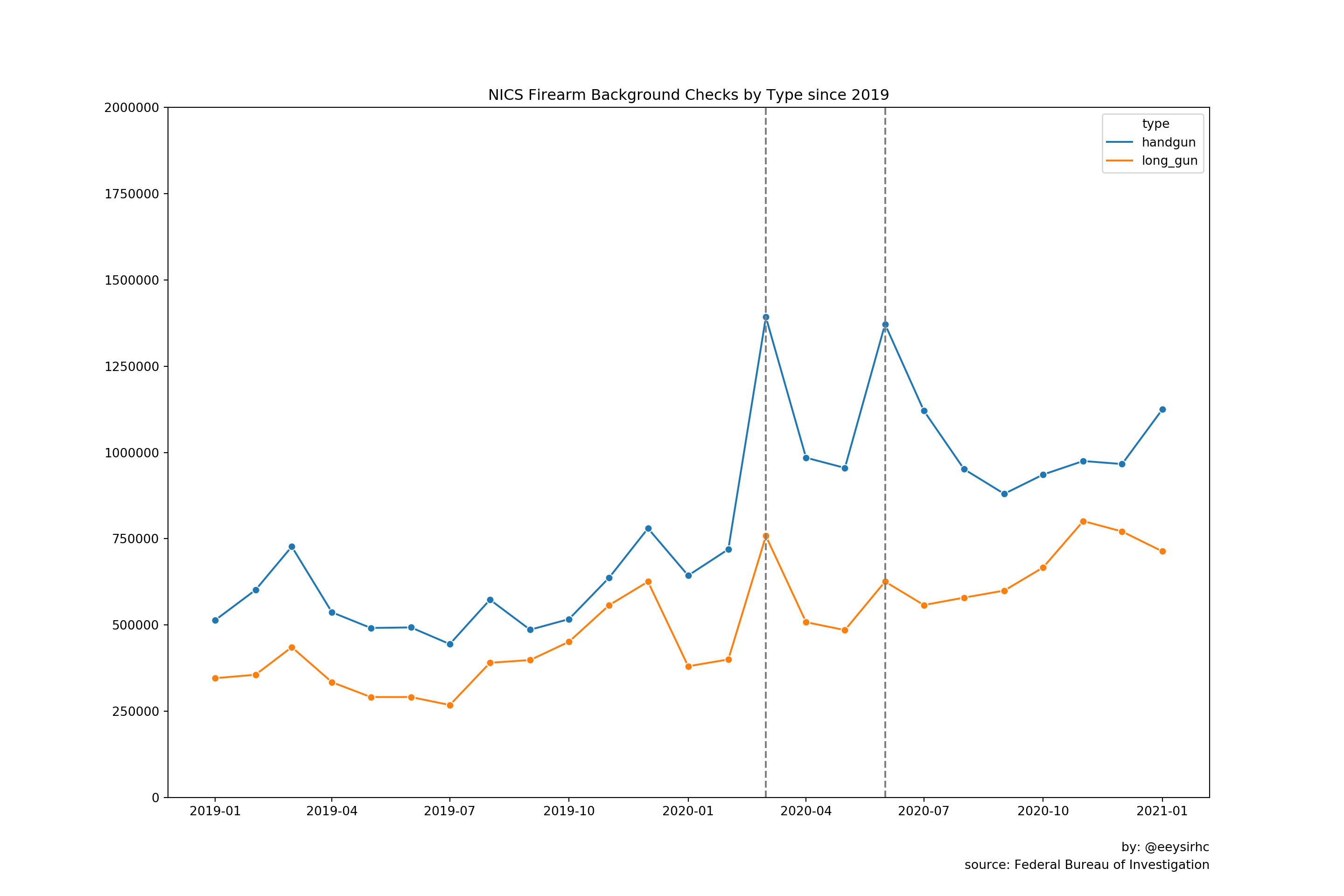
The plot above highlights two major spikes in firearm sales - especially for handguns.
- March: the coronavirus reaches the shores of the US and forces the country to go into pseudo-lockdown
- June: Black Lives Matter protests erupt across the country due to the extrajudicial killing of George Floyd
If we focus just on March there is a +92% year-over-year increase for handguns and +74% for long guns.
nics_guntype['index_year'] = pd.DatetimeIndex(nics_guntype['month']).year
nics_guntype['index_month'] = pd.DatetimeIndex(nics_guntype['month']).month
nics_guntype = nics_guntype[['month', 'handgun', 'long_gun', 'index_month']]

(nics_guntype[nics_guntype['index_month'] == 3]
    .sort_values('month', ascending=False).head())
## month handgun long_gun index_month
## 256 2020-03-01 1392677.0 758073.0 3
## 244 2019-03-01 727226.0 435698.0 3
## 232 2018-03-01 781452.0 540979.0 3
## 220 2017-03-01 751866.0 461273.0 3
## 208 2016-03-01 736630.0 430837.0 3So, how are Americans coping with 2020 thus far?
We are buying lots and lots of guns which, admittedly, is 100% expected.
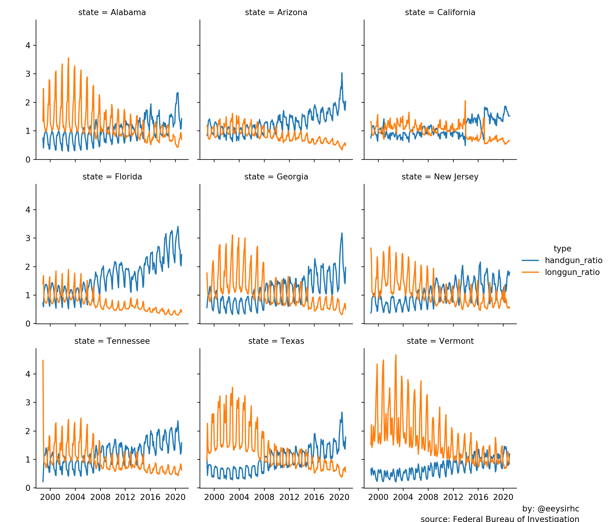
Moment of zen
And just for fun…
nics_state = (nics[['month', 'state', 'handgun', 'long_gun']]
    .groupby(['month', 'state']).agg('sum').reset_index())

nics_state['handgun_ratio'] = nics_state['handgun'] / nics_state['long_gun']
nics_state['longgun_ratio'] = nics_state['long_gun'] / nics_state['handgun']

states = ['California', 'Tennessee', 'Vermont', 'New Jersey', 'Texas', 'Arizona', 'Georgia', 'Florida', 'Alabama']

nics_state_filter = nics_state[nics_state['state'].isin(states)]

nics_state_parsed = (pd.melt(nics_state_filter, id_vars=['month', 'state'],
    value_vars=['handgun_ratio', 'longgun_ratio'], var_name='type'))

plt.figure(figsize=(15,10))

p = sns.FacetGrid(nics_state_parsed, col="state", hue="type", col_wrap=3)
p = (p.map(plt.plot, "month", "value").add_legend()
    .set_xlabels("").set_ylabels(""))
plt.figtext(0.95, 0.02, "by: @eeysirhc", horizontalalignment="right")
plt.figtext(0.95, 0.00, "source: Federal Bureau of Investigation", horizontalalignment="right")

plt.show()