Google Trends is great for understanding relative search popularity for a given keyword or phrase. However, if we wanted to explore the topics some more it is quite clunky to retrieve that data within the web interface.
Enter the gtrendsR package for #rstats and what better way to demonstrate how this works than by pulling search popularity for ramen, pho, and spaghetti (hot on the heels of my last article about ramen ratings)!
Load packages
library(tidyverse)
library(lubridate)
library(gtrendsR)
Extract Google Trends data
Maximum of five keywords at a time and let’s focus only on US search interest.
food <- gtrends(c("ramen", "pho", "spaghetti"),
               geo = c("US"))
Clean up our dataframe
food_timeseries <- as_tibble(food$interest_over_time) %>%
  mutate(date = ymd(date)) %>% # CONVERT DATE FORMAT
  filter(date < Sys.Date() - 7) # REMOVE "NOISY" DATA FROM LAST SEVEN DAYS
Quick peek at data
food_timeseries## # A tibble: 780 x 7
## date hits keyword geo time gprop category
## <date> <int> <chr> <chr> <chr> <chr> <int>
## 1 2016-02-07 15 ramen US today+5-y web 0
## 2 2016-02-14 16 ramen US today+5-y web 0
## 3 2016-02-21 16 ramen US today+5-y web 0
## 4 2016-02-28 16 ramen US today+5-y web 0
## 5 2016-03-06 16 ramen US today+5-y web 0
## 6 2016-03-13 15 ramen US today+5-y web 0
## 7 2016-03-20 17 ramen US today+5-y web 0
## 8 2016-03-27 16 ramen US today+5-y web 0
## 9 2016-04-03 17 ramen US today+5-y web 0
## 10 2016-04-10 17 ramen US today+5-y web 0
## # … with 770 more rowsGraph interest over time
food_timeseries %>%
  ggplot() +
  geom_line(aes(date, hits, color = keyword), size = 1) +
  scale_y_continuous(limits = c(0, 100)) +
  scale_color_brewer(palette = 'Set2') +
  theme_bw() +
  labs(x = NULL,
       y = "Relative Search Interest",
       color = NULL,
title = "Google Trends: interest over time (US)") 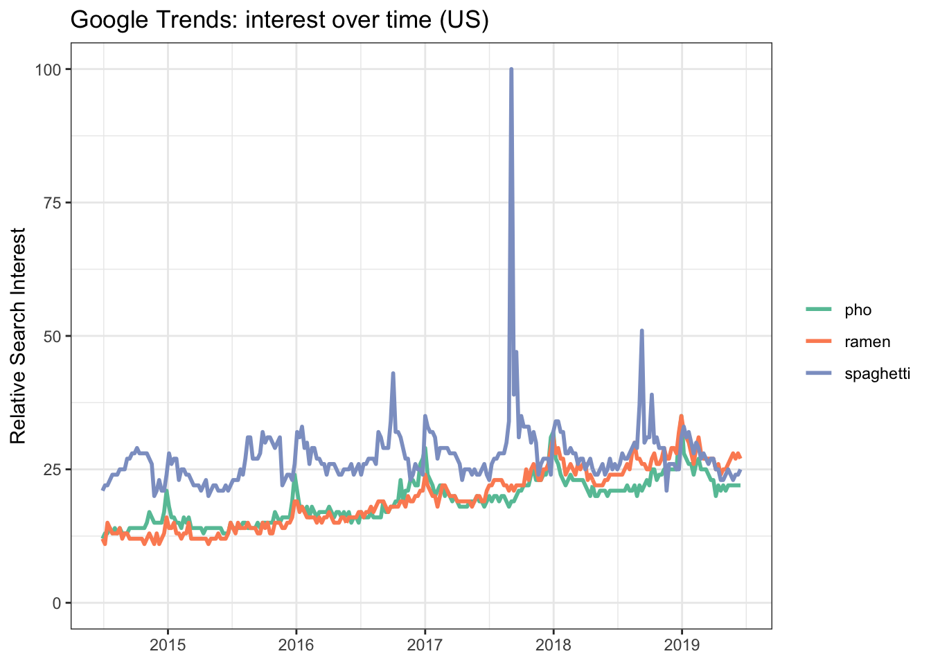
It looks like ramen has picked up traction over the last five years and even surpassed spaghetti popularity earlier this year.
I wonder what that will look like a year from now? We’ll look to using the prophet package from Facebook to forecast future popularity.
Forecasting relative search popularity
Load packages
library(prophet)Prepare the data
Let’s see how we do for ramen search popularity.
ramen_timeseries <- food_timeseries %>%
  filter(keyword == 'ramen') %>%
  select(date, hits) %>%
  mutate(date = ymd(date)) %>%
  rename(ds = date, y = hits) %>% # CONVERT COLUMN HEADERS FOR PROPHET
  arrange(ds) # ARRANGE BY DATE
Build the model
ramen_m <- prophet(ramen_timeseries)
ramen_future <- make_future_dataframe(ramen_m, periods = 365) # PREDICT 365 DAYS
ramen_ftdata <- as_tibble(predict(ramen_m, ramen_future))
Combine forecast with actuals
ramen_forecast <- ramen_ftdata %>%
  mutate(ds = ymd(ds),
         segment = case_when(ds > Sys.Date()-7 ~ 'forecast',
                             TRUE ~ 'actual'), # SEGMENT ACTUAL VS FORECAST DATA
         keyword = paste0("ramen")) %>%
  select(ds, segment, yhat_lower, yhat, yhat_upper, keyword) %>%
  left_join(ramen_timeseries) # JOIN ACTUAL DATA
Plot forecasting results
ramen_forecast %>%
  rename(date = ds,
         actual = y) %>%
  ggplot() +
  geom_line(aes(date, actual)) + # PLOT ACTUALS DATA
  geom_point(data = subset(ramen_forecast, segment == 'forecast'),
            aes(ds, yhat), color = 'salmon', size = 0.1) + # PLOT PREDICTION DATA
  geom_ribbon(data = subset(ramen_forecast, segment == 'forecast'),
            aes(ds, ymin = yhat_lower, ymax = yhat_upper),
            fill = 'salmon', alpha = 0.3) + # SHADE PREDICTION DATA REGION
  scale_y_continuous(limits = c(0,100)) +
  theme_bw() +
  labs(x = NULL, y = "Relative Search Interest",
       title = "Google Trends: interest over time for \"ramen\" (US)")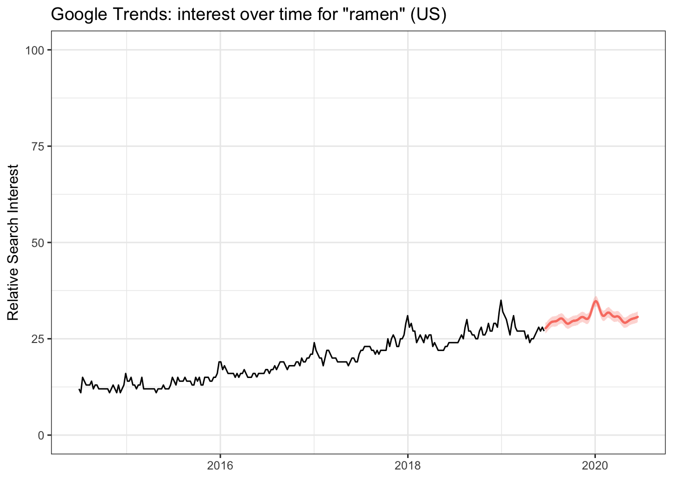
The chart above doesn’t look too bad however this is relative search popularity so we need to compare the prediction with pho and spaghetti as well.
# FUTURE NOTE: REFACTOR FOR DRY PRINCIPLES

# BUILD FORECASTING MODEL FOR PHO
pho_timeseries <- food_timeseries %>%
  filter(keyword == 'pho') %>%
  select(date, hits) %>%
  mutate(date = ymd(date)) %>%
  rename(ds = date, y = hits) %>%
  arrange(ds)

pho_m <- prophet(pho_timeseries)
pho_future <- make_future_dataframe(pho_m, periods = 365)
pho_ftdata <- as_tibble(predict(pho_m, pho_future))

pho_forecast <- pho_ftdata %>%
  mutate(ds = ymd(ds),
         segment = case_when(ds > Sys.Date()-7 ~ 'forecast',
                             TRUE ~ 'actual'),
         keyword = paste0("pho")) %>%
  select(ds, segment, yhat_lower, yhat, yhat_upper, keyword) %>%
  left_join(pho_timeseries)

# BUILD FORECASTING MODEL FOR SPAGHETTI
spaghetti_timeseries <- food_timeseries %>%
  filter(keyword == 'spaghetti') %>%
  select(date, hits) %>%
  mutate(date = ymd(date)) %>%
  rename(ds = date, y = hits) %>%
  arrange(ds)

spaghetti_m <- prophet(spaghetti_timeseries)
spaghetti_future <- make_future_dataframe(spaghetti_m, periods = 365)
spaghetti_ftdata <- as_tibble(predict(spaghetti_m, spaghetti_future))

spaghetti_forecast <- spaghetti_ftdata %>%
  mutate(ds = ymd(ds),
         segment = case_when(ds > Sys.Date()-7 ~ 'forecast',
                             TRUE ~ 'actual'),
         keyword = paste0("spaghetti")) %>%
  select(ds, segment, yhat_lower, yhat, yhat_upper, keyword) %>%
  left_join(spaghetti_timeseries)

# COMBINE ALL MODELS
keyword_forecast <- rbind(ramen_forecast, pho_forecast, spaghetti_forecast) %>%
  rename(date = ds, actual = y)
Final plot
keyword_forecast %>%
  ggplot() +
  geom_line(aes(date, actual, color = keyword), size = 1) +
  geom_ribbon(data = subset(keyword_forecast, segment == 'forecast'),
              aes(date, ymin = yhat_lower, ymax = yhat_upper, fill = keyword),
            alpha = 0.3) +
  geom_point(data = subset(keyword_forecast, segment == 'forecast'),
             aes(date, yhat, color = keyword), size = 0.1) +
  scale_y_continuous(limits = c(0,100)) +
  scale_color_brewer(palette = 'Set2') +
  scale_fill_brewer(palette = 'Set2') +
  theme_bw() +
  labs(x = NULL, y = "Relative Search Interest",
title = "Google Trends: interest over time (US)") 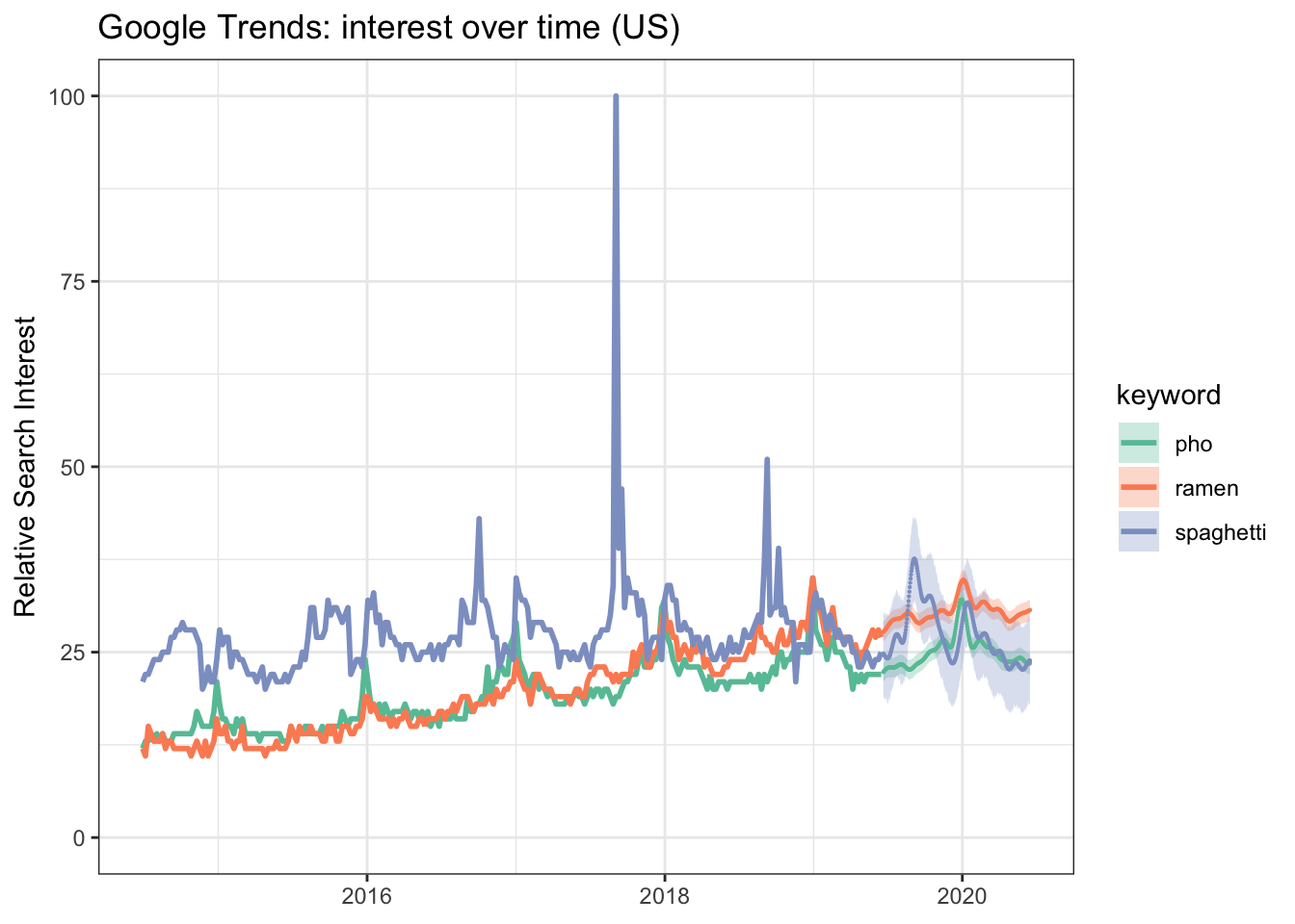
One year from now we should expect to see ramen at the top followed by pho and spaghetti fighting for a close second in terms of relative search interest.
Text mining related queries
The other awesome functionality provided by the gtrendsR package is pulling top & rising queries for each topic.
Here’s a sample result for pho:
food_related <- as_tibble(food$related_queries)

food_related %>%
  filter(keyword == 'pho')
## # A tibble: 50 x 6
## subject related_queries value geo keyword category
## <chr> <chr> <chr> <chr> <chr> <int>
## 1 100 top pho near me US pho 0
## 2 49 top pho menu US pho 0
## 3 28 top pho restaurant US pho 0
## 4 26 top pho food US pho 0
## 5 23 top pho saigon US pho 0
## 6 21 top vietnamese US pho 0
## 7 20 top vietnamese pho US pho 0
## 8 19 top pho soup US pho 0
## 9 18 top pho recipe US pho 0
## 10 17 top pho thai US pho 0
## # … with 40 more rowsWe can call it a day at this point but it would be too boring - let’s do some text mining to see if we can find any lexical nuggets.
Load packages
library(tidytext)
library(igraph)
library(ggraph)

a <- grid::arrow(type = "closed", length = unit(.15, "inches"))
I’m curious: what is the relationship of the top queries for ramen, pho and spaghetti ?
Parse data and create graph
topqueries_bigram <- food_related %>%
  filter(related_queries == 'top') %>%
  unnest_tokens(bigram, value, token = 'ngrams', n = 3) %>%
  separate(bigram, c("word1", "word2"), sep = " ") %>%
  filter(!word1 %in% stop_words$word, !word2 %in% stop_words$word) %>%
  count(word1, word2, sort = TRUE) %>%
  filter(!is.na(word1), !is.na(word2)) %>%
  graph_from_data_frame()
Plot graph
set.seed(0612)

ggraph(topqueries_bigram, layout = "fr") +
  geom_edge_link(aes(edge_alpha = n), show.legend = FALSE,
                 arrow = a, end_cap = circle(.07, 'inches')) +
  geom_node_point(color = 'steelblue', size = 3) +
  geom_node_text(aes(label = name), vjust = 1, hjust = 1) +
  theme_void() +
  labs(title = "Google Trends: top queries (US)",
       caption = "by: @eeysirhc")
Not bad - we were able to visualize how spaghetti terms are relatively different and thus further away from its soupier Asian counterparts. Moreover, we were able to sift through the nosie and identify the related terms for each topic.
Now, just for fun, what about the relationship between rising queries?
Before we build our graph we want to spice things up a bit by adding an additional layer on top of the data. In this case, varying the size and color of our nodes based on the number of word occurrences.
word_counts <- food_related %>%
  select(value) %>%
  unnest_tokens(word, value) %>%
  count(word, sort = TRUE) %>%
  filter(!word %in% stop_words$word)
Parse data and create graph
risingqueries_bigram <- food_related %>%
  filter(related_queries == 'rising') %>%
  unnest_tokens(bigram, value, token = 'ngrams', n = 3) %>%
  separate(bigram, c("word1", "word2"), sep = " ") %>%
  filter(!word1 %in% stop_words$word, !word2 %in% stop_words$word) %>%
  count(word1, word2, sort = TRUE) %>%
  filter(!is.na(word1), !is.na(word2)) %>%
  graph_from_data_frame(vertices = word_counts)
Plot graph
set.seed(0613)

ggraph(risingqueries_bigram, layout = "fr") +
  geom_edge_link(aes(edge_alpha = n), show.legend = FALSE,
                 arrow = a, end_cap = circle(.07, 'inches')) +
  geom_node_point(aes(size = n, color = n)) +
  geom_node_text(aes(label = name), vjust = 1, hjust = 1) +
  scale_color_gradient2(low = 'salmon', high = 'seagreen', midpoint = 25) +
  theme_void() +
  theme(legend.position = 'none') +
  labs(title = 'Google Trends: rising queries (US)',
caption = "by: @eeysirhc") 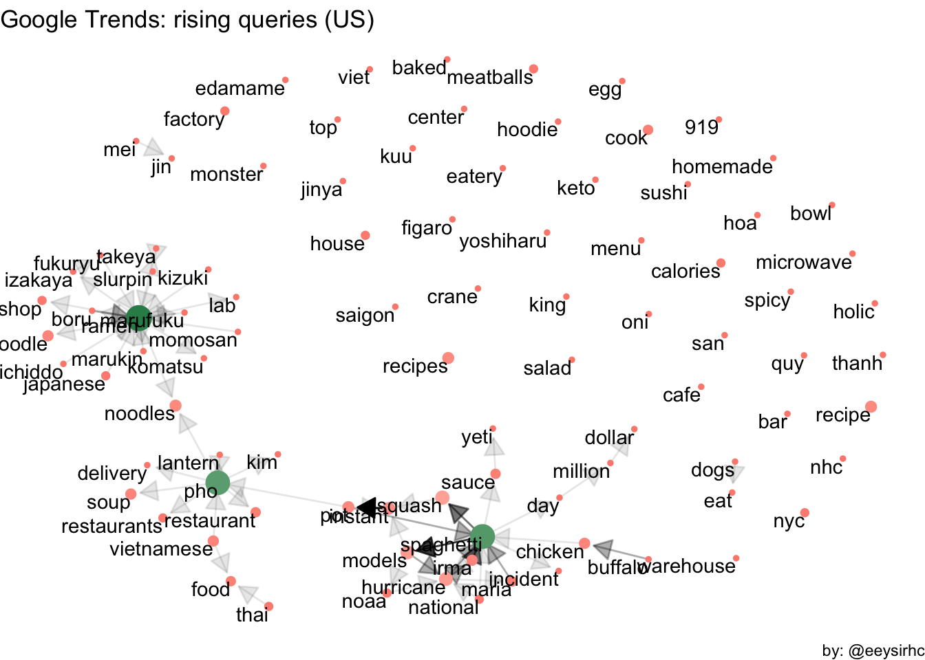
Wrapping up
You will find a million methods on how to download Google Trends data.
This is just one way to do it in R where we pulled the data, plotted historical trends, forecasted future search popularity, and even performed some light text mining to find relationship between words.