R script for the CausalImpact package

Load libraries

library(tidyverse)
library(CausalImpact)

Download (dummy) data

df <- read_csv("https://raw.githubusercontent.com/Eeysirhc/random_datasets/master/cimpact_sample_data.csv")

df %>% sample_n(5)

## # A tibble: 5 x 3
##   date       experiment_type revenue
##   <date>     <chr>             <dbl>
## 1 2020-04-02 control           309. 
## 2 2020-05-05 experiment        257. 
## 3 2020-02-29 control           928. 
## 4 2020-03-13 control           467. 
## 5 2020-03-02 experiment         35.0

Shape data

Before we can run our analysis, the CausalImpact package requires three columns:

• Date (YYYY-MM-DD)
• Response/Treatment
• Control

If your data is already structured in the above format then feel free to skip to the next section.

Otherwise, we need to massage our (dummy) data frame from a long to wide format.

df_clean <- df %>%
  dplyr::select(date, experiment_type, revenue) %>%
  pivot_wider(names_from = "experiment_type",
              values_from = "revenue") %>%
  dplyr::select(date, experiment, control)

And a quick spot check:

df_clean %>% 
  arrange(date) %>% 
  head()

## # A tibble: 6 x 3
##   date       experiment control
##   <date>          <dbl>   <dbl>
## 1 2020-02-27       21.3    235.
## 2 2020-02-28        0      407.
## 3 2020-02-29        0      928.
## 4 2020-03-01       32.7    535.
## 5 2020-03-02       35.0    664.
## 6 2020-03-03       17.5    581.

Set parameters

The code below will:

• Set the intervention start date
• How many days forward/backward to compare from start date (I suggest full 7-day weeks)
• Construct appropriate date variables

test_date <- as.Date("2020-04-23")

test_length <- 21

pre <- c(test_date-(test_length+1), test_date-1)
post <- c(test_date, (test_date+test_length))

Let’s also make sure our date differences are correct:

pre[2]-pre[1]

## Time difference of 21 days

And the post period?

post[2]-post[1]

## Time difference of 21 days

Good to go!

Run causal impact analysis

df_impact <- CausalImpact(df_clean, pre, post)

Plot results

plot(df_impact)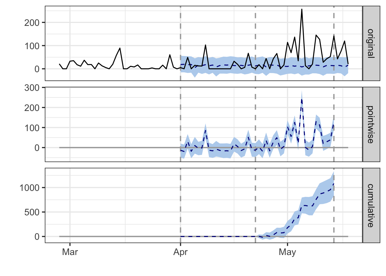

Analysis summary

summary(df_impact)

## Posterior inference {CausalImpact}
## 
##                          Average        Cumulative  
## Actual                   62             1371        
## Prediction (s.d.)        13 (5.8)       288 (127.3) 
## 95% CI                   [1.7, 24]      [37.0, 537] 
##                                                     
## Absolute effect (s.d.)   49 (5.8)       1083 (127.3)
## 95% CI                   [38, 61]       [834, 1334] 
##                                                     
## Relative effect (s.d.)   376% (44%)     376% (44%)  
## 95% CI                   [289%, 463%]   [289%, 463%]
## 
## Posterior tail-area probability p:   0.00101
## Posterior prob. of a causal effect:  99.89909%
## 
## For more details, type: summary(impact, "report")

Detailed analysis

summary(df_impact, "report")

## Analysis report {CausalImpact}
## 
## 
## During the post-intervention period, the response variable had an average value of approx. 62.33. By contrast, in the absence of an intervention, we would have expected an average response of 13.10. The 95% interval of this counterfactual prediction is [1.68, 24.43]. Subtracting this prediction from the observed response yields an estimate of the causal effect the intervention had on the response variable. This effect is 49.24 with a 95% interval of [37.90, 60.65]. For a discussion of the significance of this effect, see below.
## 
## Summing up the individual data points during the post-intervention period (which can only sometimes be meaningfully interpreted), the response variable had an overall value of 1.37K. By contrast, had the intervention not taken place, we would have expected a sum of 0.29K. The 95% interval of this prediction is [0.04K, 0.54K].
## 
## The above results are given in terms of absolute numbers. In relative terms, the response variable showed an increase of +376%. The 95% interval of this percentage is [+289%, +463%].
## 
## This means that the positive effect observed during the intervention period is statistically significant and unlikely to be due to random fluctuations. It should be noted, however, that the question of whether this increase also bears substantive significance can only be answered by comparing the absolute effect (49.24) to the original goal of the underlying intervention.
## 
## The probability of obtaining this effect by chance is very small (Bayesian one-sided tail-area probability p = 0.001). This means the causal effect can be considered statistically significant.