After two politically-charged years, Robert Mueller finally concluded his investigation on Russian interference with the 2016 presidential elections.
The outcome was a 440+ page report on their findings - the perfect candidate for some text mining.
Side note: the idea for this post came when my attempts to extract the PDF text proved unsuccessful because it was locked in an unsearchable version.
As a consequence of that I did a little tweet mining instead:too busy to read all 400+ pages of the #muellerreport but apparently not busy enough to do some text/tweet mining with #rstats
— Christopher Yee (@Eeysirhc) April 18, 2019
according to this network graph though I should definitely check out page 290 pic.twitter.com/RPiahsrg9A
Forutnately there are people much smarter than me and were able to produce a user-friendly format of the redacted report.
Get the data
library(tidyverse)
library(tidytext)

mueller_report_raw <- read_csv("https://raw.githubusercontent.com/gadenbuie/mueller-report/master/mueller_report.csv")

mueller_report <- mueller_report_raw
Clean the data
# REMOVE NON-CHAR AND NON-NUMBERS
mueller_report$text <- str_replace_all(mueller_report$text,"[^a-zA-Z\\s]", " ")

# CONVERT TO LOWER CASE
mueller_report$text <- str_to_lower(mueller_report$text)

# REMOVE EXTRA WHITE SPACE
mueller_report$text <- str_replace_all(mueller_report$text,"[\\s]+", " ")
Calculate and plot TF-IDF for every 40 pages
data(stop_words)

mueller_report %>%
  mutate(page_group = 39 * (page %/% 39)+ 1,   # CREATE GROUPS PER 40 PAGES
         page_group = as.factor(page_group)) %>%
  group_by(page_group) %>%
  unnest_tokens(word, text) %>%
  anti_join(stop_words) %>%
  count(word, sort = TRUE) %>%
  bind_tf_idf(word, page_group, n) %>%
  arrange(desc(tf_idf)) %>%
  group_by(page_group) %>%
  top_n(10) %>%
  ungroup() %>%
  mutate(word = reorder(word, tf_idf)) %>%
  ggplot() +
  geom_col(aes(word, tf_idf),
           show.legend = FALSE,
           fill = 'steelblue') +
  facet_wrap(~page_group, ncol = 3, scales = "free") +
  coord_flip() +
  theme_light() +
  theme(panel.grid.major = element_blank(),
        panel.grid.minor = element_blank(),
        axis.text.x = element_blank()) +
  labs(x = NULL,
       y = NULL,
       title = "Redacted Mueller Report: top keywords per 40 pages based on TF-IDF",
       caption = "Author: @eeysirhc")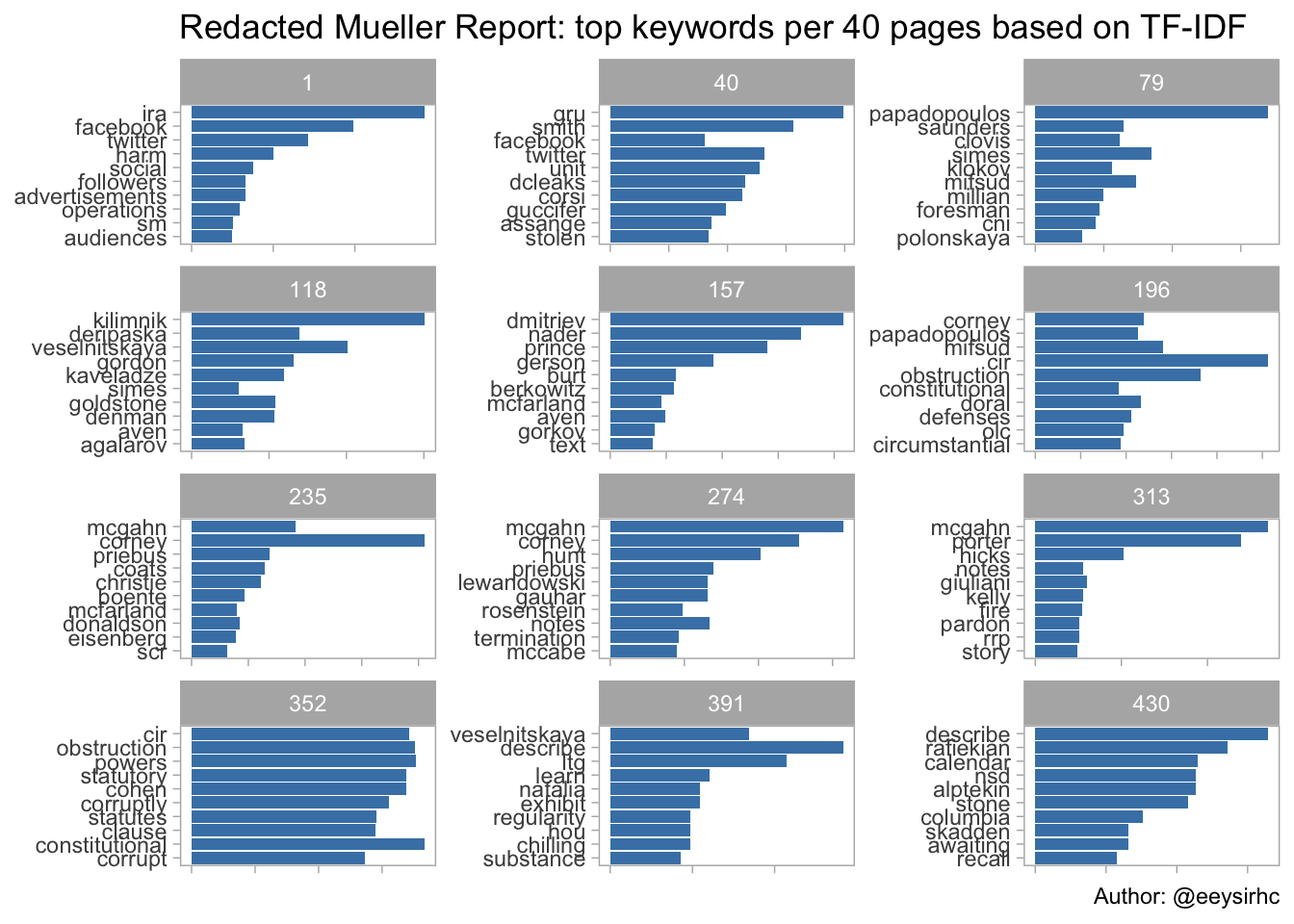
Following each page group gives an idea of the history, events and conclusions from the Mueller report.
Create the document term matrix for topic modeling
library(topicmodels)

desc_dtm <- mueller_report %>%
  group_by(page) %>%
  unnest_tokens(word, text) %>%
  anti_join(stop_words) %>%
  count(word, sort = TRUE) %>%
  cast_dtm(page, word, n)

desc_lda <- LDA(desc_dtm, k = 12, control = list(seed = 1234))   # 12 WAS BEST FIT AFTER I TRIED 9 AND 24

top_terms <- tidy(desc_lda) %>%
  group_by(topic) %>%
  top_n(10, beta) %>%
  ungroup() %>%
  arrange(topic, -beta)
Process and plot the LDA topic models
top_terms %>%
  mutate(term = reorder(term, beta)) %>%
  group_by(topic, term) %>%
  arrange(desc(beta)) %>%
  ungroup() %>%
  mutate(term = factor(paste(term, topic, sep = "__"),
                       levels = rev(paste(term, topic, sep = "__")))) %>%
  ggplot(aes(term, beta)) +
  geom_col(show.legend = FALSE, fill = 'seagreen', alpha = 0.8) +
  coord_flip() +
  scale_x_discrete(labels = function(x) gsub("__.+$", "", x)) +
  labs(title = "Redacted Mueller Report: top 20 keywords in each LDA topic",
       x = NULL, y = NULL,
       caption = "Author: @eeysirhc") +
  facet_wrap(~ topic, ncol = 3, scales = "free") +
  theme_light() +
  theme(panel.grid.major = element_blank(),
        panel.grid.minor = element_blank(),
        axis.text.x = element_blank())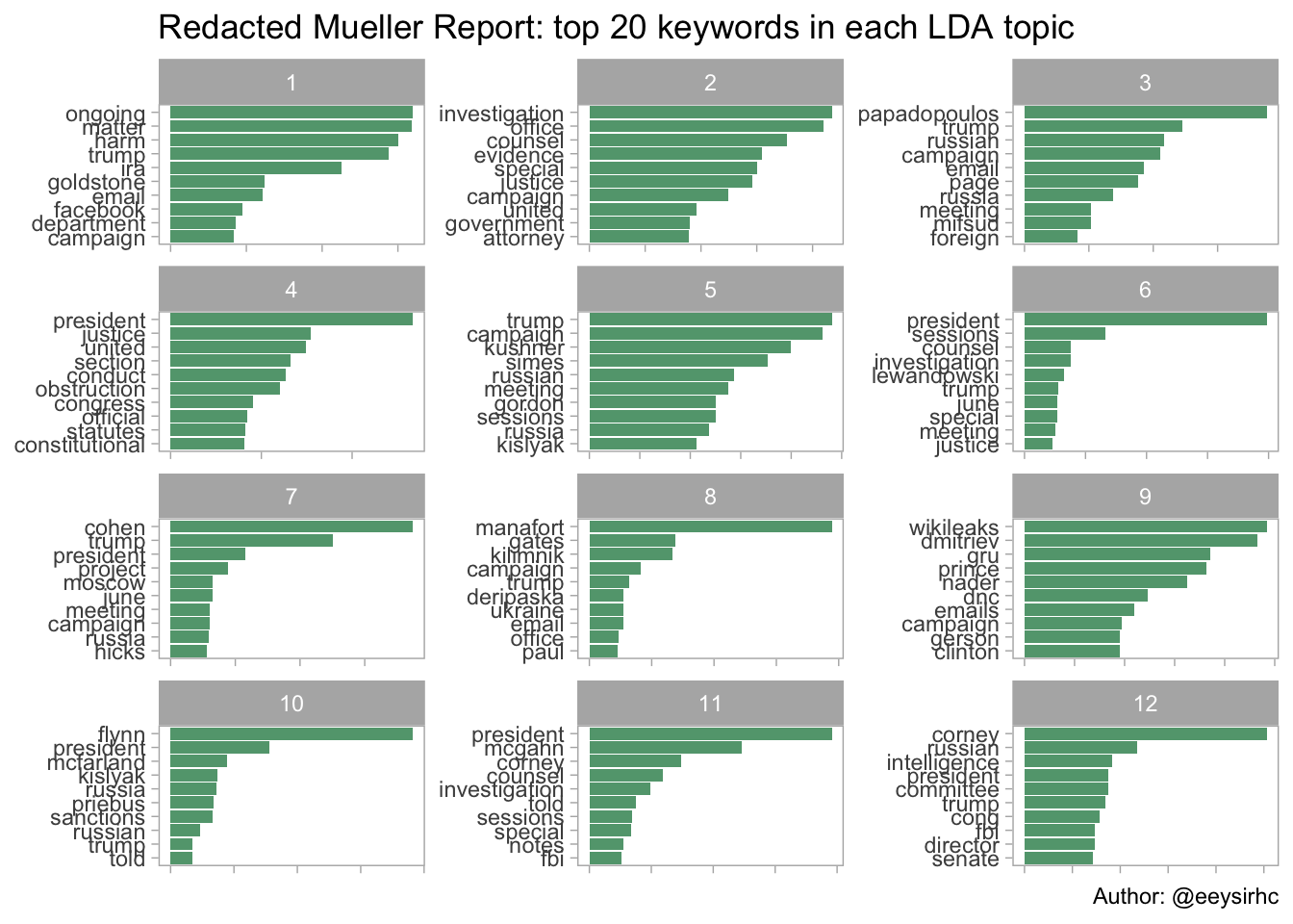
With latent Dirichlet allocation, or LDA, we now have a sense of the major topics and the associated keywords in the redacted report.
In other words (no pun intended), we are now speed reading with data science.