Analyzing data for #tidytuesday week of 12/4/2018 (source)
# LOAD PACKAGES AND PARSE DATA
library(tidyverse)
library(scales)
library(RColorBrewer)
library(forcats)
library(tidytext)
library(stringr)

articles_raw <- read_csv("https://raw.githubusercontent.com/rfordatascience/tidytuesday/master/data/2018/2018-12-04/medium_datasci.csv")

articles <- articles_raw
Who are the top 10 authors in terms of total articles published?
top_authors <- articles %>%
  select(author) %>%
  group_by(author) %>%
  count() %>%
  arrange(desc(n)) %>%
  na.omit() %>%
  head(10)

top_authors %>%
  ggplot() +
  geom_col(aes(reorder(author, n), n),
           fill = "darkslategray4",
           alpha = 0.8) +
  coord_flip() +
  theme_bw() +
  labs(x = "",
       y = "",
       title = "Top 10 authors on Medium in terms of total articles published")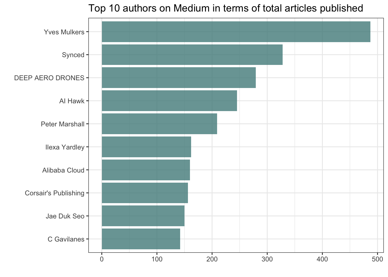
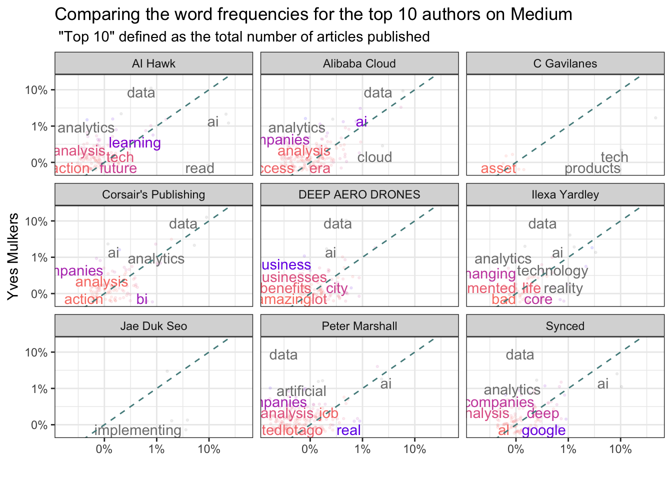
Are there differences in words used between the titles and subtitles?
Clean up data before we text mine the top 10 authors
data(stop_words)

tidy_authors <-
  articles %>%
  inner_join(top_authors) %>%
  select(title, subtitle, author) %>%
  na.omit() %>%
  mutate(text = paste(title, " ", subtitle)) %>%
  select(author, text) %>%
  unnest_tokens(word, text) %>%
  anti_join(stop_words)
Calculate proportions and plot graph
tidy_authors %>%
  group_by(author) %>%
  mutate(word = str_extract(word, "[a-z']+")) %>%
  count(word, sort = TRUE) %>%
  mutate(proportion = n / sum(n)) %>%
  select(-n) %>%
  spread(author, proportion) %>%
  gather(author, proportion, `AI Hawk`:`Synced`) %>%
  ggplot(aes(x=proportion, y=`Yves Mulkers`, color = abs(`Yves Mulkers` - proportion))) +
  geom_jitter(alpha = 0.1,
              size = 0.5,
              width = 0.25,
              height = 0.25) +
  geom_text(aes(label = word),
            check_overlap = TRUE,
            vjust = 1,
            hjust = 1) +
  geom_abline(color = "darkslategray4",
              linetype = 2) +
  scale_color_gradient(limits = c(0, 0.01),
                       low = "salmon",
                       high = "blue") +
  scale_x_log10(labels = percent_format(round(1))) +
  scale_y_log10(labels = percent_format(round(1))) +
  labs(y = "Yves Mulkers",
       x = "",
       title = "Comparing the word frequencies for the top 10 authors on Medium",
       subtitle = " \"Top 10\" defined as the total number of articles published") +
  theme_bw() +
  theme(legend.position = "none") +
  facet_wrap(~author, ncol = 3)