Analyzing data for #tidytuesday week of 01/01/2019 (source)
# LOAD PACKAGES AND PARSE DATA
library(tidyverse)
library(scales)
library(RColorBrewer)
library(forcats)
library(tidytext)
library(topicmodels)

tweets_raw <- as_tibble(readRDS("rstats_tweets.rds"))
Parse data and identify top users
# IDEA BEHIND THIS IS TO FILTER OUT BOTS

# FIND TOP USERS
top_interactions <- tweets_raw %>%
  select(screen_name, favorite_count, retweet_count) %>%
  group_by(screen_name) %>%
  summarize(favorite = sum(favorite_count),
            retweet = sum(retweet_count)) %>%
  group_by(screen_name) %>%
  mutate(total = sum(favorite, retweet)) %>%
  arrange(desc(total)) %>%
  head(12)

# JOIN TOP USERS WITH RAW DATASET
tweets <- tweets_raw %>%
  inner_join(top_interactions, by='screen_name')

# FINAL DATA PROCESSING
tweets_parsed <- tweets %>%
  select(screen_name, text) %>%
  group_by(screen_name) %>%
  unnest_tokens(word, text) %>%
  anti_join(stop_words) %>%
  filter(!grepl("https|t.co|http|bit.ly|kindly|goo.gl|rstats|amp", word)) # REMOVE EXTRA STOP WORDS
What are the most significant keywords for each #rstats Twitter user?
tweets_tfidf <- tweets_parsed %>%
  count(screen_name, word, sort = TRUE) %>%
  ungroup() %>%
  bind_tf_idf(word, screen_name, n)

tweets_tfidf %>%
  filter(!near(tf, 1)) %>%
  arrange(desc(tf_idf)) %>%
  group_by(screen_name) %>%
  distinct(screen_name, word, .keep_all = TRUE) %>%
  top_n(10, tf_idf) %>%
  ungroup() %>%
  mutate(word = factor(word, levels = rev(unique(word)))) %>%
  ggplot(aes(word, tf_idf, fill = screen_name)) +
  geom_col(show.legend = FALSE) +
  facet_wrap(~screen_name, ncol = 4, scales = "free") +
  coord_flip() +
  theme_light() +
  labs(x = "",
       y = "",
       title = "Highest TF-IDF words for top #rstats Twitter users",
       caption = "Source: data from {rtweet} package") +
  scale_fill_brewer(palette = 'Paired')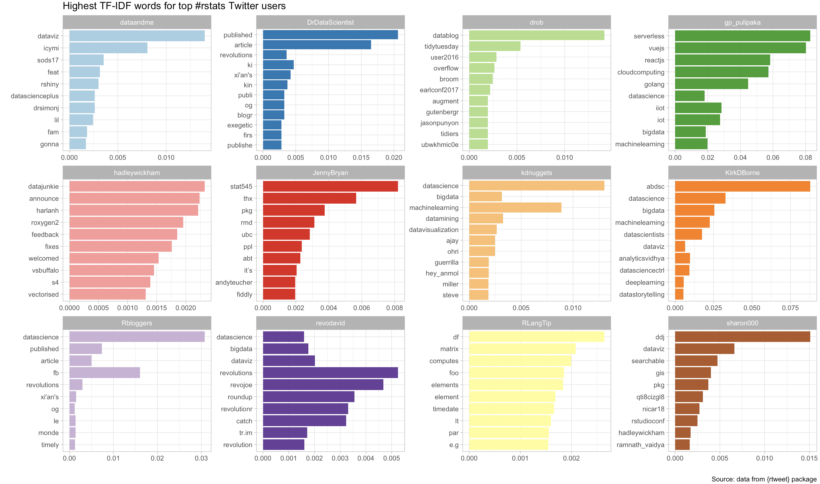
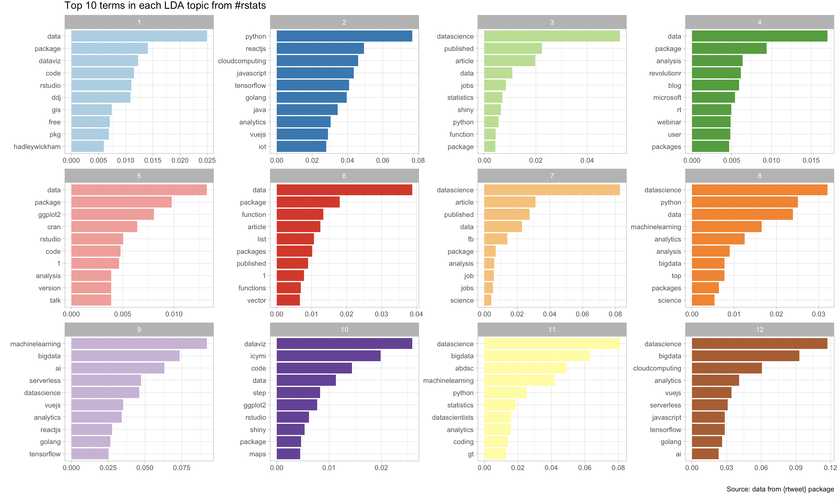
What are the topics and highest proability keywords for each?
tweet_words <- tweets_parsed %>%
  count(screen_name, word, sort = TRUE) %>%
  ungroup()

tweet_dtm <- tweet_words %>%
  cast_dtm(screen_name, word, n)

tweets_lda <- LDA(tweet_dtm, k=12, control = list(seed = 2019))

tidy_lda <- tidy(tweets_lda)

top_terms <- tidy_lda %>%
  group_by(topic) %>%
  top_n(10, beta) %>%
  ungroup() %>%
  arrange(topic, -beta)

top_terms %>%
  mutate(term = reorder(term, beta)) %>%
  group_by(topic, term) %>%
  arrange(desc(beta)) %>%
  ungroup() %>%
  mutate(term = factor(paste(term, topic, sep = "__"),
                       levels = rev(paste(term, topic, sep = "__")))) %>%
  ggplot(aes(term, beta, fill = as.factor(topic))) +
  geom_col(show.legend = FALSE) +
  coord_flip() +
  scale_x_discrete(labels = function(x) gsub("__.+$", "", x)) +
  scale_fill_brewer(palette = 'Paired') +
  labs(title = "Top 10 terms in each LDA topic from #rstats",
       caption = "Source: data from {rtweet} package",
       x = "",
       y = "") +
  theme_light() +
  facet_wrap(~topic, ncol = 4, scales = "free")