Analyzing data for #tidytuesday week of 1/15/2019 (source)
# LOAD PACKAGES AND PARSE DATA
library(tidyverse)
library(RColorBrewer)
library(forcats)
library(scales)
library(ebbr)

launches_raw <- read_csv("https://raw.githubusercontent.com/rfordatascience/tidytuesday/master/data/2019/2019-01-15/launches.csv")

launches <- launches_raw %>%
  filter(launch_year >= '1960')
Distribution of the most space launches over time?
countries <- launches %>%
  count(state_code, sort = TRUE) %>%
  filter(n >= 100)

launches %>%
  inner_join(countries) %>%
  # INCOMING NASTY IFELSE CODE (NEED TO REFACTOR)
  mutate(state_code = ifelse(state_code == 'RU', 'Russia / Soviet Union',
                             ifelse(state_code == 'SU', 'Russia / Soviet Union',
                                    ifelse(state_code == 'US', 'United States',
                                           ifelse(state_code == 'CN', 'China',
                                                  ifelse(state_code == 'IN', 'India',
                                                         ifelse(state_code == 'F', 'France',
                                                                ifelse(state_code == 'J', 'Japan', state_code)))))))) %>%
  ggplot() +
  geom_density(aes(launch_year, fill = state_code, color = state_code),
               alpha = 0.2) +
  theme_light() +
  scale_color_brewer(palette = 'Set1') +
  scale_fill_brewer(palette = 'Set1') +
  labs(x = "",
       y = "",
       title = "Distribution of space launches over time by country",
       subtitle = "Minimum of 100 launches",
       caption = "Source: The Economist",
       fill = "Country",
       color = "Country") +
  scale_y_continuous(labels = percent_format(round(1)))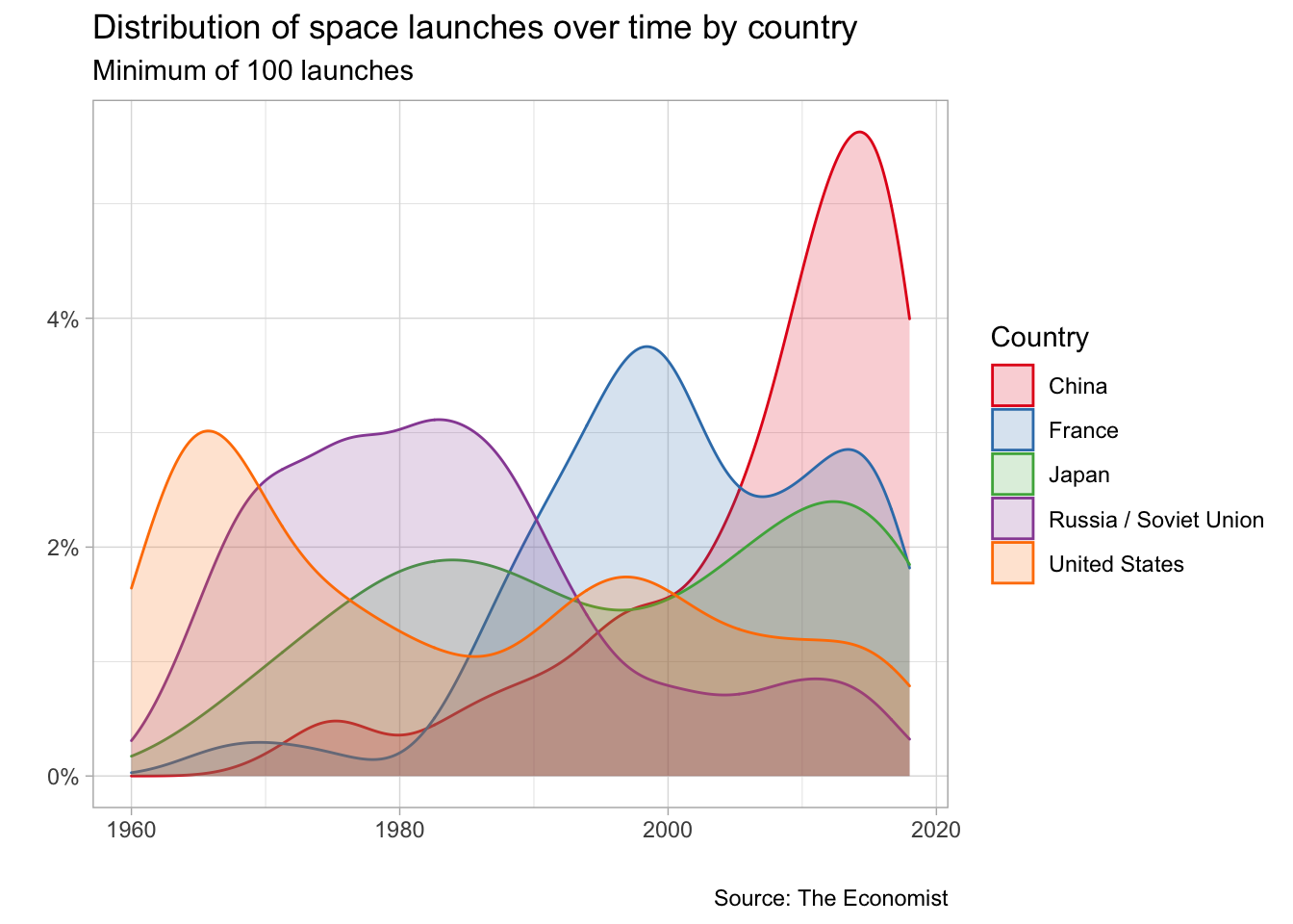
Who has a better success rate: private, startup or states ?
launches %>%
  mutate(category = ifelse(category == 'O', 1, 0)) %>%
  select(launch_year, agency_type, category) %>%
  group_by(launch_year, agency_type) %>%
  summarize(success = sum(category),
            total = n(),
            rate = success / total) %>%
  ungroup() %>%
  add_ebb_estimate(success, total) %>%
  mutate(agency_type = str_to_title(agency_type)) %>%
  ggplot() +
  geom_line(aes(launch_year, .fitted, color = agency_type),
            size = 1) +
  geom_ribbon(aes(x = launch_year, ymin = .low, ymax = .high, fill = agency_type),
              alpha = 0.1) +
  theme_light() +
  scale_fill_brewer(palette = 'Set1') +
  scale_color_brewer(palette = 'Set1') +
  labs(x = "",
       y = "",
       caption = "Source: The Economist",
       title = "Success rate of space launches by type",
       subtitle = "Empirical Bayes rate @ 95% credible interval",
       color = "Type",
       fill = "Type") +
  scale_y_continuous(labels = percent_format(round(1)),
                     limits = c(0,1))
## Warning: `data_frame()` is deprecated as of tibble 1.1.0.
## Please use `tibble()` instead.
## This warning is displayed once every 8 hours.
## Call `lifecycle::last_warnings()` to see where this warning was generated.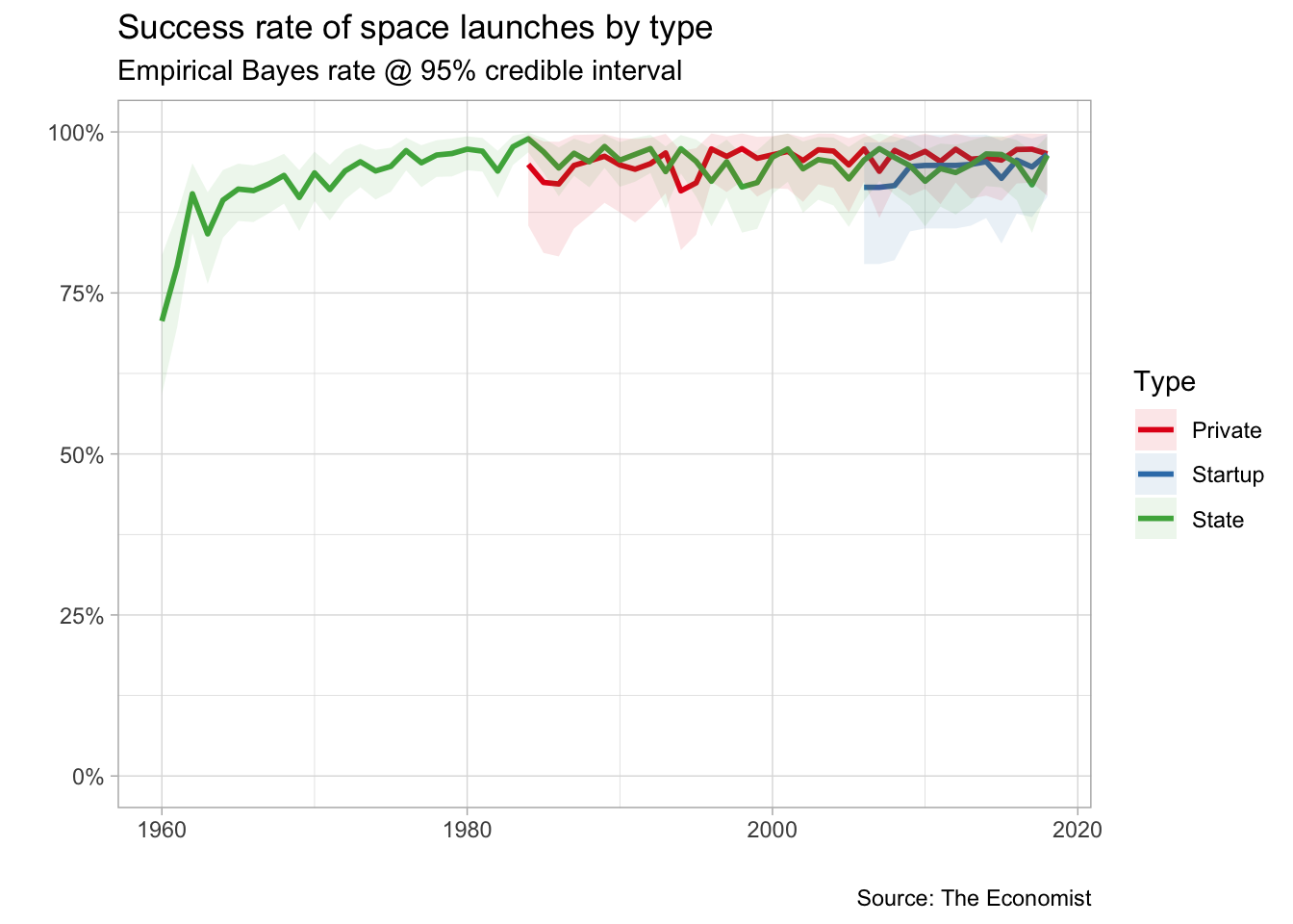
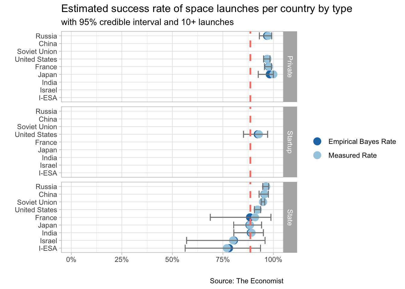
Success rate for each country by agency type ?
# APPLY EMPIRICAL BAYESIAN STATS TO DATASET
launches_parsed <- launches %>%
  mutate(category = ifelse(category == 'O', 1, 0),
         agency_type = str_to_title(agency_type)) %>%
  select(launch_year, state_code, agency_type, category) %>%
  group_by(state_code, agency_type) %>%
  summarize(success = sum(category),
         total = n(),
         rate = success / total) %>%
  ungroup() %>%
  add_ebb_estimate(success, total)

# PLOT THE GRAPH
launches_parsed %>%
  filter(total >= 10) %>%
  select("Empirical Bayes Rate"=.fitted,
         "Measured Rate"=.raw,
         everything()) %>%
  gather(key, value, `Empirical Bayes Rate`:`Measured Rate`) %>%
    # INCOMING NASTY IFELSE CODE (NEED TO REFACTOR)
  mutate(state_code = ifelse(state_code == 'RU', 'Russia',
                             ifelse(state_code == 'SU', 'Soviet Union',
                                    ifelse(state_code == 'US', 'United States',
                                           ifelse(state_code == 'CN', 'China',
                                                  ifelse(state_code == 'IN', 'India',
                                                         ifelse(state_code == 'F', 'France',
                                                                ifelse(state_code == 'J', 'Japan',
                                                                       ifelse(state_code == 'IL', 'Israel', state_code))))))))) %>%
  ggplot() +
  geom_point(aes(x=reorder(state_code, value), y=value, color = key), size = 4) +
  geom_errorbar(aes(x = state_code, ymin = .low, ymax = .high), size = 0.5, color = "gray50") +
  geom_hline(data=launches_parsed, aes(yintercept = median(.fitted)), color = 'salmon', linetype = 'dashed', size = 1) +
  coord_flip() +
  theme_light() +
  scale_y_continuous(labels = percent_format(round(1)),
                     limits = c(0,1)) +
  labs(x = "",
       title = "Estimated success rate of space launches per country by type",
       subtitle = "with 95% credible interval and 10+ launches",
       y = "",
       caption = "Source: The Economist",
       color = "") +
  scale_color_brewer(palette = 'Paired', direction = -1) +
  facet_grid(agency_type~.)