Analyzing data for #tidytuesday week of 01/08/2019 (source)
# LOAD PACKAGES AND PARSE DATA
library(knitr)
library(tidyverse)
library(RColorBrewer)
library(forcats)
library(lubridate)
library(broom)

tv_data_raw <- read_csv("https://raw.githubusercontent.com/rfordatascience/tidytuesday/master/data/2019/2019-01-08/IMDb_Economist_tv_ratings.csv")

tv_data <- tv_data_raw
Prepare the data for k-means clustering
tv_data_summarized <- tv_data %>%
  group_by(title, genres, date) %>%
  summarize(min_rating = min(av_rating),
            avg_rating = mean(av_rating),
            max_rating = max(av_rating),
            min_share = min(share),
            avg_share = mean(share),
            max_share = max(share)) %>%
  ungroup()

kclust_data <- tv_data_summarized %>%
  select(-title, -genres, -date)

kclust_results <- kmeans(kclust_data, center = 9)
Check output data (boxplot)
# CHECK OUTPUT DATA
tv_data_summarized %>%
  left_join(augment(kclust_results, kclust_data)) %>%
  mutate(title = factor(title)) %>%
  group_by(.cluster) %>%
  ggplot() +
  geom_boxplot(aes(.cluster, avg_rating, fill = .cluster),
               show.legend = FALSE,
               alpha = 0.5) +
  theme_light() +
  labs(x = "Cluster #",
       y = "Average Rating",
       caption = "Source: The Economist",
       title = "Average rating distribution for each cluster assignment") +
  scale_fill_brewer(palette = 'Paired')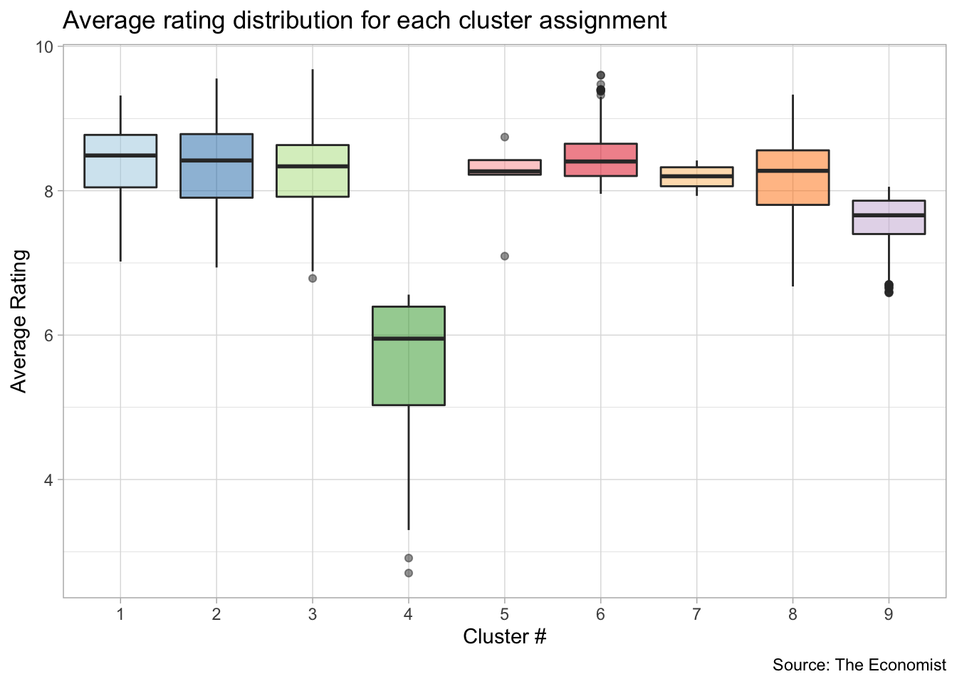
Check outputdata (scatterplot)
tv_data_summarized %>%
  left_join(augment(kclust_results, kclust_data)) %>%
  mutate(title = factor(title)) %>%
  group_by(.cluster) %>%
  ggplot(aes(avg_rating, log10(avg_share)+1, color = .cluster)) +
  geom_point(alpha = 0.7, size = 3, show.legend = FALSE) +
  theme_light() +
    labs(x = "Average Rating",
       y = "Share (log10)",
       caption = "Source: The Economist",
       title = "Relationship between Average Rating and Shares by cluster assignment") +
  scale_fill_brewer(palette = 'Paired')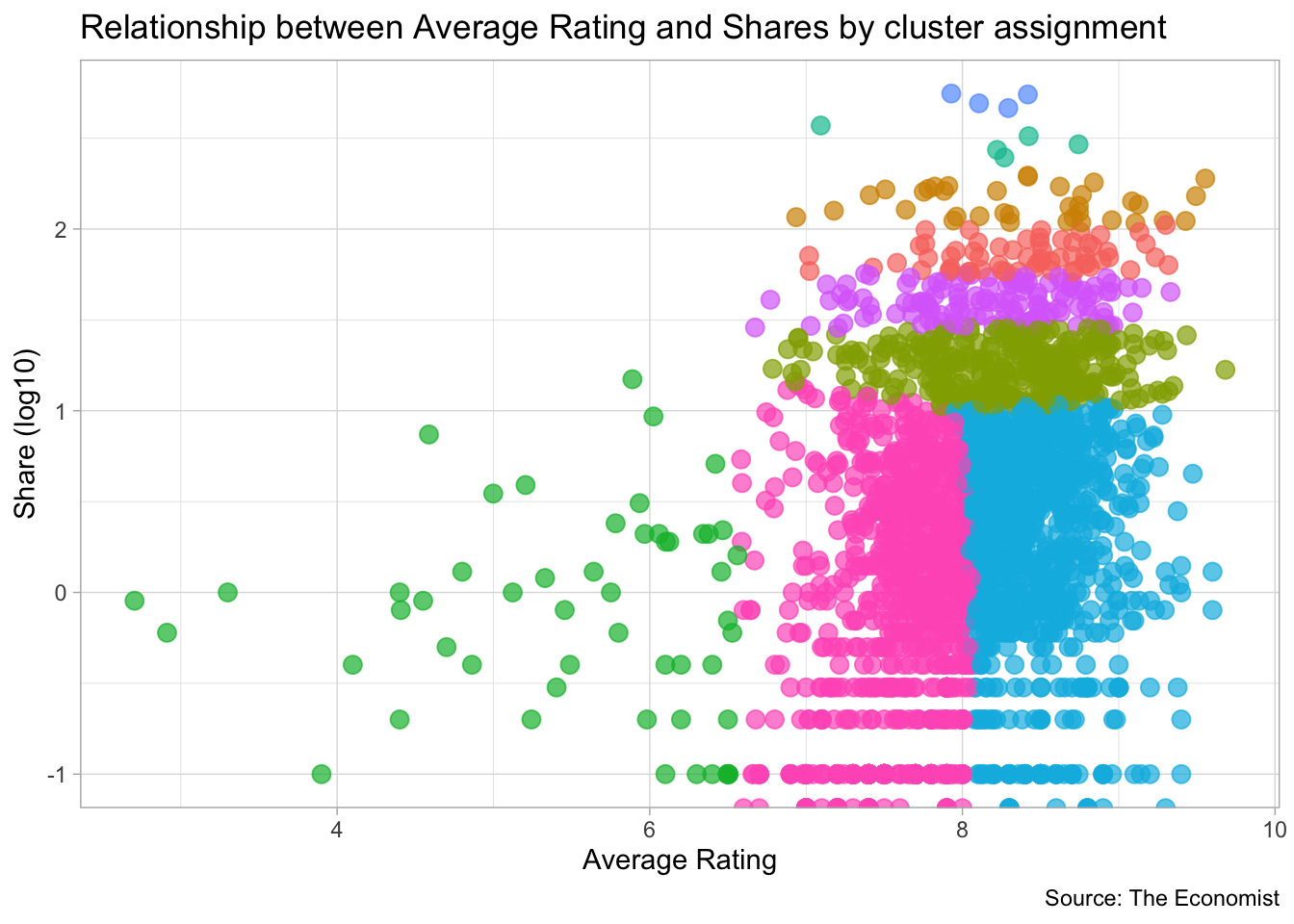
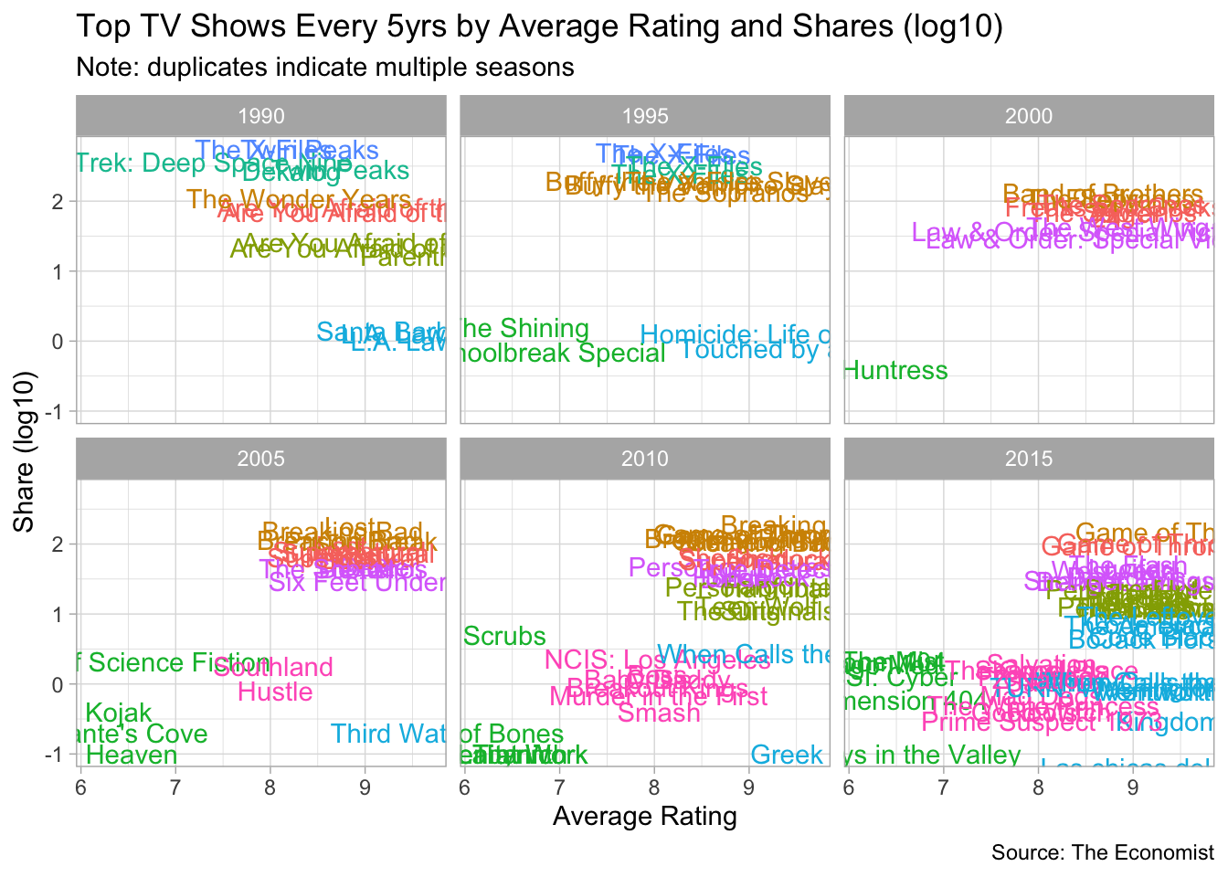
Finalize the plot
tv_data_summarized %>%
  left_join(augment(kclust_results, kclust_data)) %>%
  mutate(title = factor(title),
         five_years = 5 * (year(date) %/% 5 )) %>%
  group_by(.cluster) %>%
  top_n(20, avg_rating) %>%
  ggplot(aes(avg_rating, log10(avg_share)+1, label = title, color = .cluster)) +
  geom_text(show.legend = FALSE) +
  facet_wrap(~five_years) +
  theme_light() +
  labs(x = "Average Rating",
       y = "Share (log10)",
       caption = "Source: The Economist",
       title = "Top TV Shows Every 5yrs by Average Rating and Shares (log10)",
       subtitle = "Note: duplicates indicate multiple seasons")