Changelog
- Originally published on September 10th, 2019
- Built a Shiny app for this
- Full code can be found on GitHub
One of my favorite online marketers, (the) Glen Allsopp, tweeted the following:
Over the past few weeks I've went through every site in the Inc. 5000. My mind has been blown multiple times. Don't click if you're easily distracted. Enjoy! https://t.co/mHVK8rvb9X pic.twitter.com/BoEb3qQ7LZ
— Glen Allsopp (@ViperChill) August 27, 2019
The public spreadsheet contains four fields:
- Inc.com URL
- URLs (company website)
- Revenue
- 3-Year-Growth
Although helpful I thought it would be interesting to explore the additional variables found on each company’s INC profile page.
Thus, I fired up R and scaped the list of URLs to answer the question: which industries were surveyed the most and how much revenue did they generate in 2019?
tl;dr
Load packages
library(tidyverse)
library(rvest) # SIMPLE WEB SCRAPING
Get URLs from CSV
inc5000 <- read_csv("inc5000_fastest_growing_companies.csv") %>%
  rename(urls = `Inc.com URL`,
         website = URLs)
Base R format
We temporarily need to move out of the tidyverse and leverage base R for the next step.
company_urls <- inc5000$urls Loop function
A for loop is required to gather our data with the following order of operations:
- Take URL from list
- Crawl the page
- Extract the page elements we want
- Store into data frame
- Rinse and repeat from step 1
# INITIALIZE DATA FRAME
company_raw <- data.frame()

for (page_url in company_urls){
  print(page_url)

  # RETRIEVE INC5000 PROFILE PAGE
  page <- read_html(page_url)

  # PARSE REVENUE
  revenue_millions <- page %>%
    html_nodes(xpath = '//*/section[1]/div[3]/dl[1]/dd') %>%
    html_text() %>%
    str_replace(" Million", "") %>% # STRIP 'MILLIONS' FROM DATA VALUE
    str_replace("\\$", "") # STRIP $ SIGN FROM DATA VALUE

  # PARSE INDUSTRY
  industry <- page %>%
    html_nodes(xpath = '//*/section[1]/div[3]/dl[3]/dd') %>%
    html_text()

 # PARSE YEAR FOUNDED
  year_founded <- page %>%
    html_nodes(xpath = '//*/section[1]/div[3]/dl[5]/dd') %>%
    html_text()

  # PARSE EMPLOYEE COUNT
  employees <- page %>%
    html_nodes(xpath = '//*/section[1]/div[3]/dl[6]/dd') %>%
    html_text()

  # TEMP TO STORE LOOP DATA
  temp_df <- data.frame(page_url, revenue_millions, industry, year_founded, employees)

  # COMBINE TEMP WITH ALL DATA
  company_raw <- rbind(company_raw, temp_df)
}
Data cleaning
Ideally, we want to separate our data collection from our data processing but I did not anticipate “billions” to show up in the parse revenue step of our loop.
We will leave it as is though to illustrate the ease with which we can clean data in R, specifically the tidyverse.
# BRING BACK TO TIDYVERSE
company_data <- company_raw %>%
  as_tibble()

# EXTRACT 'BILLION' VALUES AND CONVERT TO MILLIONS
billions <- company_data %>%
  filter(grepl(" Billion", revenue_millions)) %>%
  mutate(revenue_millions = str_replace(revenue_millions, " Billion", ""),
         revenue_millions = as.numeric(as.character(revenue_millions)),
         revenue_millions = revenue_millions*1000)

# CONVERT 'MILLION' VALUES TO NUMERICAL FORMAT
company_data <- company_data %>%
  filter(!grepl(" Billion", revenue_millions)) %>%
  mutate(revenue_millions = as.numeric(as.character(revenue_millions)))

# JOIN OUR SANITIZED DATASET
company_data <- rbind(company_data, billions)
Summarize data
With our cleaned dataset we can finally answer the question: how much revenue did each industry generate in 2019 and how many companies were surveyed?
company_parsed <- company_data %>%
  group_by(industry) %>%
  summarize(revenue_millions = sum(revenue_millions),
            count = n()) %>%
  ungroup() %>%
  filter(!is.na(revenue_millions)) %>%
  mutate(pct_count = count / sum(count),
         pct_revenue = revenue_millions / sum(revenue_millions),
revenue_billions = revenue_millions / 1000) | industry | revenue_billions | count | pct_revenue | pct_count |
|---|---|---|---|---|
| Health | 38.9890 | 360 | 0.1650677 | 0.0718276 |
| Consumer Products & Services | 23.2248 | 323 | 0.0983268 | 0.0644453 |
| Construction | 20.4304 | 354 | 0.0864962 | 0.0706305 |
| Logistics & Transportation | 18.7815 | 184 | 0.0795152 | 0.0367119 |
| Government Services | 14.0165 | 236 | 0.0593417 | 0.0470870 |
| Business Products & Services | 13.9789 | 490 | 0.0591825 | 0.0977654 |
| Human Resources | 11.4535 | 156 | 0.0484907 | 0.0311253 |
| Retail | 10.8481 | 163 | 0.0459276 | 0.0325219 |
| Financial Services | 9.5650 | 239 | 0.0404953 | 0.0476856 |
| Software | 9.2791 | 457 | 0.0392849 | 0.0911812 |
| Advertising & Marketing | 9.0369 | 489 | 0.0382595 | 0.0975658 |
| Real Estate | 6.4951 | 195 | 0.0274983 | 0.0389066 |
| IT Management | 6.2604 | 276 | 0.0265047 | 0.0550678 |
| Energy | 6.2551 | 77 | 0.0264822 | 0.0153631 |
| Manufacturing | 5.9942 | 179 | 0.0253776 | 0.0357143 |
| Food & Beverage | 5.0617 | 127 | 0.0214297 | 0.0253392 |
| Telecommunications | 3.3042 | 79 | 0.0139890 | 0.0157622 |
| Insurance | 3.1245 | 69 | 0.0132282 | 0.0137670 |
| Engineering | 2.6693 | 81 | 0.0113010 | 0.0161612 |
| IT System Development | 2.5352 | 121 | 0.0107333 | 0.0241421 |
| Education | 1.4515 | 69 | 0.0061452 | 0.0137670 |
Unsurprisingly, the Health industry comes out on top with a whopping $39Bn - nearly 1.7x more than the runner up Consumer Products & Services.
In terms of companies surveyed, we have Business Products & Services at #1 with 490 companies and a very close second for the Advertising & Marketing industry at 489.
Keeping it real
Rather than a signal of the US economy, it's more a sign of which types of companies care about this (paid) PR exposure. Inc 5000 is a badge to show-off at agencies and software companies. Less so in other markets. It's not surprising that Health is the real winner (in the US) 🙂
— Rob Kerry (@robkerry) September 11, 2019
Visualize data
The tabulated data above is a little difficult to interpret so we’ll plot our results instead.
library(ggrepel)

company_parsed %>%
  ggplot(aes(pct_count, pct_revenue, label = industry)) +
  geom_point() +
  geom_label_repel() +
  geom_abline(color = 'salmon', lty = 'dashed') +
  scale_x_continuous(labels = scales::percent_format(round(1)),
                     limits = c(0, .1)) +
  scale_y_continuous(labels = scales::percent_format(round(1)),
                     limits = c(0, .2)) +
  labs(x = "% of Total Companies", y = "% of Total Revenue",
       title = "Inc.5000 Fastest Growing Private Companies of 2019",
       subtitle = "Compares the number of companies surveyed to total revenue generated per industry",
       caption = "by:@eeysirhc\nsource:@viperchill") +
  theme_minimal()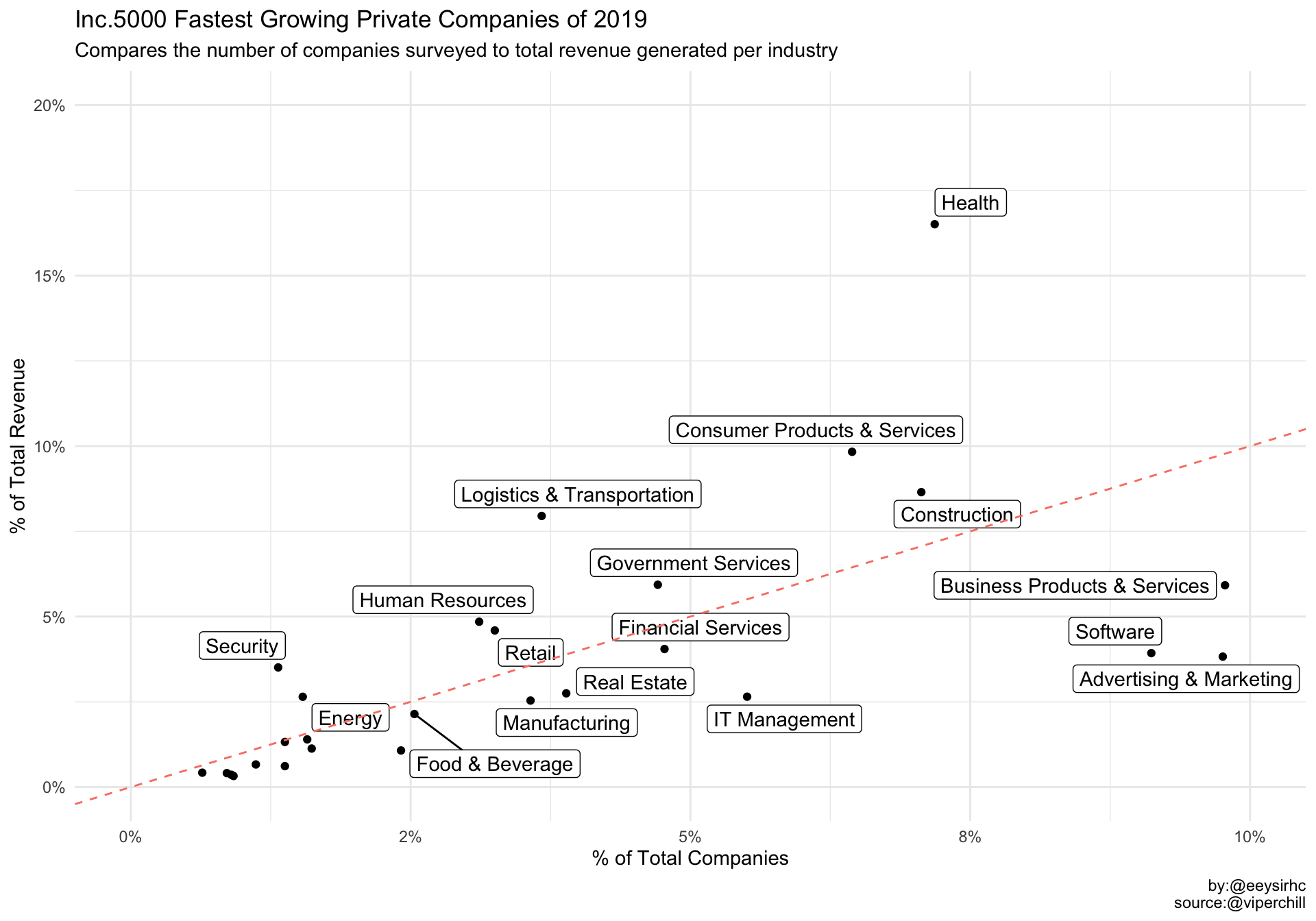
We are pretty much done but there may be instances where we want data values to be accessible for users. Luckily, the {plotly} package is our answer.
Chart interactivity
library(plotly)

plot_ly(data = company_parsed,
        x = ~pct_count,
        y = ~pct_revenue,
        mode = "scatter",
        type = "scatter",
        size = 10,
        color = ~industry,
        colors = 'Set1',
        hoverinfo = "text",
        text = ~paste("<b>Industry:</b> ",industry,
                     "<br><b>Total Companies:</b> ", count,
                      "<br><b>Total Revenue ($Bn):</b> ", revenue_billions),
        showlegend = FALSE) %>%
  layout(xaxis = list(title = "% of Total Companies",
                      tickformat = "%"),
         yaxis = list(title = "% of Total Revenue",
                      tickformat = "%"))
Wrapping up
In my next article we’ll take this a step further by building our own Shiny app. If you’re feeling adventurous then you can use some starter code here or checkout a barebones version for the US housing price index.
As always, if you enjoyed this or found it helpful please share over your favorite internet medium!