Aside from the base bid, Google SEM campaign performance can be influenced by contextual signals from the customer. These include but are not limited to: device, location, gender, parental status, household income, etc.
For this post we’ll focus on ad schedule (or intraday) and visualize how time of day and day of week is performing.
Load data
library(tidyverse)

# ANONYMIZED SAMPLE DATA
df <- read_csv("https://raw.githubusercontent.com/Eeysirhc/random_datasets/master/intraday_performance.csv")
Spot check our data
df %>%
  sample_n(20)
## # A tibble: 20 x 5
## account day_of_week hour_of_day roas conv_rate
## <chr> <chr> <dbl> <dbl> <dbl>
## 1 Account 3 Tuesday 5 0.509 0.0183
## 2 Account 2 Friday 4 1.11 0.0401
## 3 Account 2 Sunday 11 1.07 0.0309
## 4 Account 3 Saturday 18 1.09 0.0301
## 5 Account 1 Thursday 19 0.303 0.0165
## 6 Account 1 Tuesday 8 0.362 0.0230
## 7 Account 2 Saturday 4 0.722 0.0340
## 8 Account 3 Friday 10 0.653 0.00844
## 9 Account 2 Wednesday 8 0.448 0.0262
## 10 Account 1 Saturday 9 0.858 0.0467
## 11 Account 1 Saturday 18 0.266 0.0136
## 12 Account 1 Saturday 8 0.871 0.0349
## 13 Account 2 Friday 14 0.546 0.0196
## 14 Account 1 Sunday 5 0.0444 0.00889
## 15 Account 3 Wednesday 21 0.530 0.0248
## 16 Account 1 Tuesday 16 0.801 0.0451
## 17 Account 2 Monday 2 0.884 0.0230
## 18 Account 2 Wednesday 19 0.772 0.0275
## 19 Account 3 Monday 21 0.444 0.0367
## 20 Account 1 Tuesday 3 0 0Clean data
Convert to factors
The day_of_week is a character and time_of_day is a double data type. We need to transform them to factors so they don’t surprise us later.
df_clean <- df %>%
  mutate(day_of_week = as.factor(day_of_week),
         hour_of_day = as.factor(hour_of_day))
Reorder day of week
If we plot our chart now it won’t be correct because day_of_week will not be arranged properly from Sunday to Saturday format.
levels(df_clean$day_of_week)## [1] "Friday" "Monday" "Saturday" "Sunday" "Thursday" "Tuesday"
## [7] "Wednesday"We can quickly refactor with a few lines of code:
df_clean$day_of_week <- factor(df_clean$day_of_week,
                               levels = c("Saturday", "Friday", "Thursday",
                                          "Wednesday", "Tuesday", "Monday", "Sunday"))
Let’s check to make sure it did what we wanted:
levels(df_clean$day_of_week)## [1] "Saturday" "Friday" "Thursday" "Wednesday" "Tuesday" "Monday"
## [7] "Sunday"Plot our results
df_clean %>%
  ggplot(aes(hour_of_day, day_of_week, fill = conv_rate)) +
  geom_tile(color = 'white') +
  scale_fill_gradient2(low = 'grey', mid = 'white', high = 'steelblue') +
  labs(y = NULL, x = "Hour of Day", fill = "Conversion Rate") +
theme_minimal() 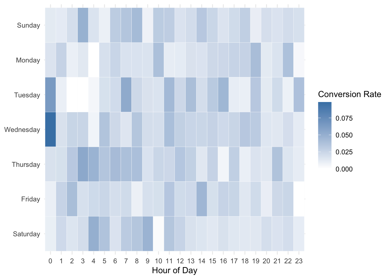
We can quickly see from this visualization that Tuesday & Wednesdays at midnight the conversion rate is 7% or higher. Conversely, 10AM on Saturday has a conversion rate close to the 0% range.
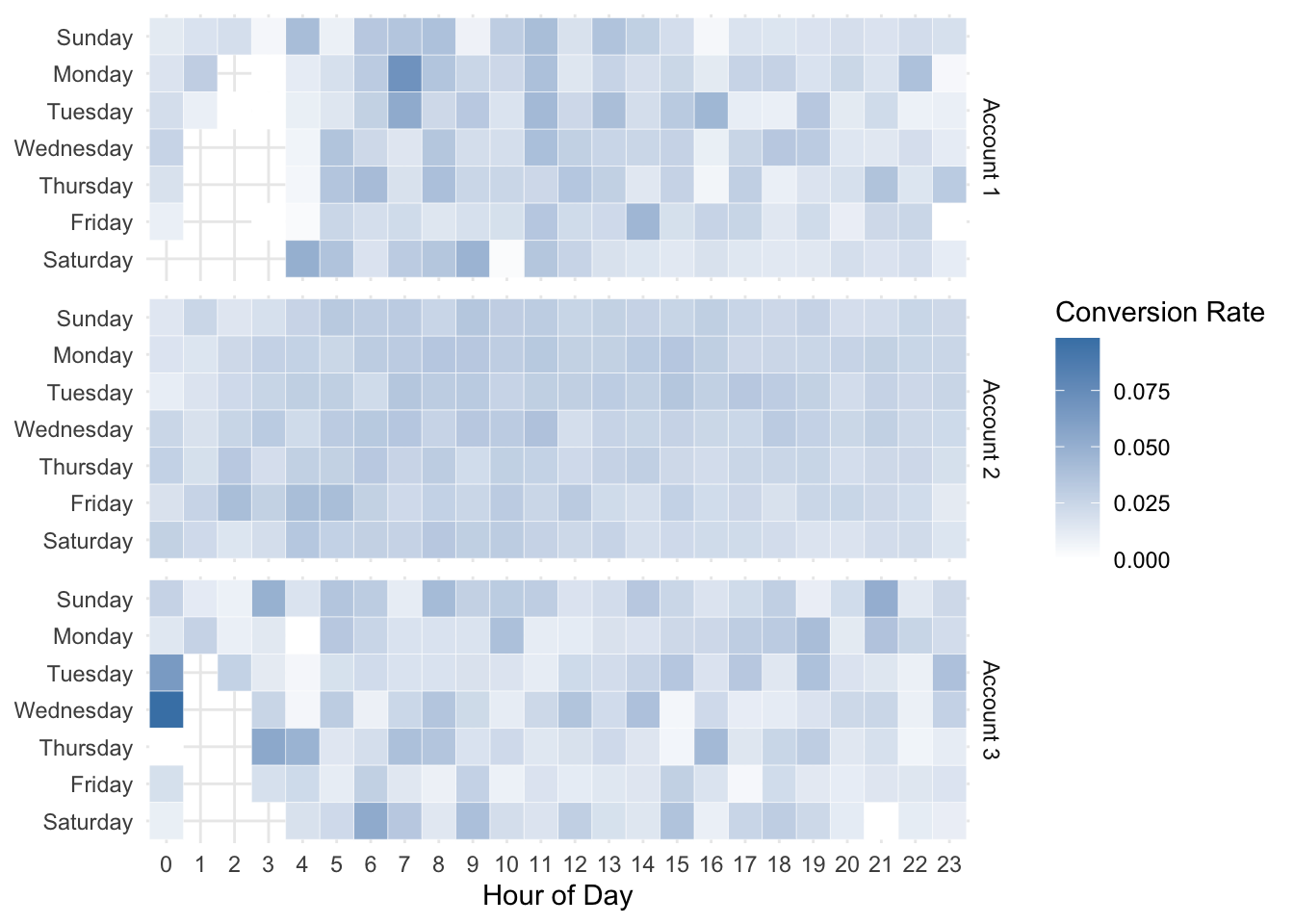
With this insight we can then amplify or dampen our intraday bid modifiers to improve overall campaign efficiencies.
And for the love of data…
…segment!
df_clean %>%
  ggplot(aes(hour_of_day, day_of_week, fill = conv_rate)) +
  geom_tile(color = 'white') +
  scale_fill_gradient2(low = 'grey', mid = 'white', high = 'steelblue') +
  labs(y = NULL, x = "Hour of Day", fill = "Conversion Rate") +
  theme_minimal() +
  facet_grid(account ~ .)