If you are like me then it’s very likely you share your Netflix account with multiple users.
If you are also like me then it’s very likely you would be curious about how your Netflix viewing activity coompares and contrasts to all the parasites on your account!
In this post we’ll leverage #rstats to visualize what that will look like.
Load packages
Let’s fire up our favorite packages.
library(tidyverse)
library(lubridate)
library(igraph)
library(ggraph)
library(tidygraph)
library(influenceR)
Download data
With the exception of my own viewing activity (I’m not ashamed!), I have provided anonymized Netflix viewing data from a few family and friends for you to follow along.
netflix_views_raw <- read_csv("https://raw.githubusercontent.com/Eeysirhc/netflix_views/master/netflix_views.csv")

netflix_views <- netflix_views_raw
Peek at our raw dataset
We can draw a random sample from our dataset to see what we are working with.
netflix_views %>%
  sample_n(10)
## # A tibble: 10 x 3
## Title Date user
## <chr> <chr> <chr>
## 1 The Umbrella Academy: Season 1: We Only See Each Other at W… 2/17/19 Chris
## 2 High Society 2/16/19 Chris
## 3 Kaze No Stigma: Season 1: The One to be Protected 2/26/12 A_sibli…
## 4 Luck-Key 7/4/18 Chris
## 5 Law & Order: Special Victims Unit: The Sixth Year: Intoxica… 11/21/… A_sibli…
## 6 Elfen Lied: Annihilation 3/5/12 A_sibli…
## 7 Imposters: Season 1: Ladies and Gentlemen, the Doctor Is In 4/29/19 Chris
## 8 Waiting for Forever 2/7/12 A_sibli…
## 9 Spartacus: Blood and Sand: Sacramentum Gladiatorum 3/27/11 A_sibli…
## 10 Arrow: Season 2: Broken Dolls 10/9/14 A_sibli…A couple data processing steps immediately spring to mind:
- Title is going to be messy if we do not canonicalize to the base name
- For the User column we can replace the dummy values so it’s easier to interpret later
Transform the data
Title - extract only the name of the show or movie
As always, we’ll take a quick look at the data.
netflix_views %>%
  select(Title) %>%
  tail() # ONLY LOOK AT THE LAST FEW ROWS OF DATA
## # A tibble: 6 x 1
## Title
## <chr>
## 1 Johnny Test: Season 3: Johnny Long Legs / Johnny Test in Outer Space
## 2 Johnny Test: Season 2: 00-Johnny / Johnny of the Jungle
## 3 Johnny Test: Season 2: Johnnyland / Johnny's Got a Brand New Dad
## 4 DreamWorks Happy Holidays from Madagascar: Volume 1: Madagascar Penguins in a…
## 5 Teen Beach Movie
## 6 KnockoutWe can then clean up our Title variable with the separate function.
netflix_views %>%
  select(Title) %>%
  tail() %>%
  separate(Title, c("title"), sep = ":", extra ='drop')
## # A tibble: 6 x 1
## title
## <chr>
## 1 Johnny Test
## 2 Johnny Test
## 3 Johnny Test
## 4 DreamWorks Happy Holidays from Madagascar
## 5 Teen Beach Movie
## 6 KnockoutWhat we did with the above was drop everything after the first colon to remove season number along with its corresponding episode name.
User - replace fake values with…..fake names
How do we know what we need to change? We can do a quick count on the User column.
netflix_views %>%
  count(user, sort = TRUE)
## # A tibble: 5 x 2
## user n
## <chr> <int>
## 1 A_sibling 5302
## 2 B_sibling 1742
## 3 D_sibling 960
## 4 Chris 923
## 5 C_sibling 97The above result informs us we need to change four of those dummy values so we’ll use a combination of mutate and case_when to achieve that.
netflix_views %>%
  sample_n(10) %>%
  select(user) %>%
  mutate(user = case_when(user == 'A_sibling' ~ "Apple",
                          user == 'B_sibling' ~ "Banana",
                          user == 'C_sibling' ~ "Cherry",
                          user == 'D_sibling' ~ "Dragon Fruit",
                          TRUE ~ user)) # THIS SAYS: IF NOTHING ELSE THEN USE THE ORIGINAL VALUE
## # A tibble: 10 x 1
## user
## <chr>
## 1 Dragon Fruit
## 2 Apple
## 3 Apple
## 4 Apple
## 5 Apple
## 6 Apple
## 7 Dragon Fruit
## 8 Apple
## 9 Banana
## 10 AppleDid it do what we wanted ?
netflix_views %>%
  #sample_n(10) %>% COMMENT THIS PORTION OUT SO WE DON'T TAKE A SAMPLE
  select(user) %>%
  mutate(user = case_when(user == 'A_sibling' ~ "Apple",
                          user == 'B_sibling' ~ "Banana",
                          user == 'C_sibling' ~ "Cherry",
                          user == 'D_sibling' ~ "Dragon Fruit",
                          TRUE ~ user)) %>%
  count(user, sort = TRUE)
## # A tibble: 5 x 2
## user n
## <chr> <int>
## 1 Apple 5302
## 2 Banana 1742
## 3 Dragon Fruit 960
## 4 Chris 923
## 5 Cherry 97Putting it all together - #tidyverse style
netflix_clean <- netflix_views %>%
  select(Date, user, Title) %>% # REARRANGE COLJUMNS
  separate(Title, c("title"), sep = ":", extra ='drop') %>%
  mutate(user = case_when(user == 'A_sibling' ~ "Apple",
                          user == 'B_sibling' ~ "Banana",
                          user == 'C_sibling' ~ "Cherry",
                          user == 'D_sibling' ~ "Dragon Fruit",
                          TRUE ~ user)) %>%
  mutate(Date = mdy(Date)) %>%
  filter(Date >= Sys.Date() - 730)  # FILTER WITHIN THE PAST TWO YEARS
And let’s validate our work:
netflix_clean## # A tibble: 261 x 3
## Date user title
## <date> <chr> <chr>
## 1 2019-04-29 Chris Imposters
## 2 2019-04-29 Chris Imposters
## 3 2019-04-29 Chris Imposters
## 4 2019-04-28 Chris Imposters
## 5 2019-04-28 Chris Imposters
## 6 2019-04-28 Chris Imposters
## 7 2019-04-28 Chris Imposters
## 8 2019-04-28 Chris Imposters
## 9 2019-04-28 Chris Imposters
## 10 2019-04-28 Chris Imposters
## # … with 251 more rowsNow that we are done cleaning our data we can finally build our network graph.
In Data Science, 80% of time spent prepare data, 20% of time spent complain about need for prepare data.
— Big Data Borat (@BigDataBorat) February 27, 2013
Build network graph
netflix_graph <- netflix_clean %>%
  count(user, title, sort = TRUE) %>% # COUNT THE NUMBER OF VIEWS PER USER BY TITLE
  filter(n >= 10) %>% # FILTER OUT LOW VOLUME DATA
  as_tbl_graph(directed = FALSE) %>%
  mutate(group = group_infomap(),
         neighbors = centrality_degree(),
         center = node_is_center(),
         dist_to_center = node_distance_to(node_is_center()),
         keyplayer = node_is_keyplayer(k = 5)) %>%
  activate(edges) %>%
  filter(!edge_is_multiple()) %>%
  mutate(centrality_e = centrality_edge_betweenness())
If you want more details on the above then I encourage you to check out this amazing intro to the ggraph package.
Visualize network graph
ggraph(netflix_graph, layout = 'kk') +
  geom_edge_link(alpha = 0.5, color = 'grey54') +
  geom_node_point(aes(color = factor(group)), size = 3, show.legend = FALSE) +
  geom_node_text(aes(label = name), size = 3, repel = TRUE) +
  scale_color_brewer(palette = "Set1") +
  theme_void() +
  labs(caption = "by: @eeysirhc")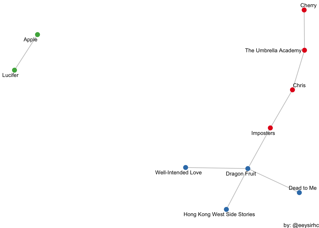
Wrapping up
Now it’s your turn - where do you lie in this network graph based on your own Netflix viewing activity? Do we watch similar TV shows or not really? How do you compare & contrast against your family and friends? What happens if you change the threshold from 10 to 20?
Don’t hesitate to share your results on Twitter!