Just like the natural world SEO traffic adheres to a Power Law, more commonly known as the long-tail or the 80-20 rule for you MBAs. Applying this to search, it means approximately 80% of your organic traffic is attributed to the top 20% of your keywords.
When you visualize this type of data though an inherent problem occurs…

…the number of visits for the head terms far exceed that of the torso and tail keywords, thus rendering the graph useless. And if you wanted a YoY comparison of your SEO performance?

No actionable insight - a fallacy of linear graphs.
Introducing Logarithmic Charts
The solution to this problem is plotting the data on a logarithmic scale where it observes Zipf’s Law. This mathematical concept states that…
…given some corpus of natural language utterances, the frequency of any word is inversely proportional to its rank in the frequency table.
In other words, your highest traffic driving keyword will occur twice as often as the second term, three times as often as the third highest traffic one and so forth.
Putting our newfound knowledge to use we can graph the YoY traffic data on a log-log plot.
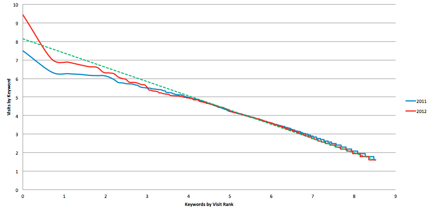
We now have a clear picture of this website’s organic search performance for the last two years where there is a noticeable jump for head term traffic in 2012 (red line) when compared to 2011 (blue line) as it surpasses the theory of Zipf’s Law (green dotted line). The long-tail traffic (Rank 5-9) for the site is holding up fairly well so my subsequent SEO strategy would focus around bolstering their torso keyword portfolio (Rank 2-4).
Overall though the graph indicates a strong year of SEO success if I dare say so myself!
Logarithmic Charting in MS Excel
Now it’s your turn to give it a shot!
1) Extract organic visits and keyword data from your web analytics package of choice (you may want to exclude not provided).
2) Insert three additional columns for Rank, Log(Rank) and Log(Visits).

3) Assuming your keyword Visits are in descending order, fill the first cell in the Rank column with the number 1, second cell with number 2 and so on.

4) In the Log(Rank) column, use the =LN function for the corresponding Rank cell.

5) Similarly, use the =LN function on the Log(Visits) column as well for the respective keyword Visits data.

6) Plot the two logarithmic columns on a “Smooth Marked Scatter” plot.

7) Add a trendline to represent Zipf’s Law.

8) Make the graph sexy.
9) Analyze.
10) Win.
Caveats
There are a couple things to keep in mind here. The first is this usually works best for medium to high traffic websites so incidentally the graph will look “better” with more data. The other is you are optimizing for “known keywords” so anything beyond page 2 is virtually invisible.
Going Deeper into the Rabbit Hole
Your analysis doesn’t have to and shouldn’t stop at the top-level because any SEO worth their salt knows you need to bucket your data to extrapolate any real insight. For example, you can plot your organic traffic by product type keywords and formulate your strategy there.

What can you take away from the graph above? Which product type would you recommend this site to optimize? If optimization is required, which keyword category (head, torso or tail) would you suggest?
Have at it and let me know what you think. Any and all types of feedback is welcomed in the comments below!