The differences between this unsanctioned #tardythursday and the official #tidytuesday:
- These will publish on Thursday (obviously)
- The dataset will come from a completely different week of TidyTuesday
- For a surprise, I’ll code with either #rstats or python (similar to #makeovermonday)
Load modules
import pandas as pd
import seaborn as sns
import matplotlib.pyplot as plt
Download and parse data
df_raw=pd.read_csv("https://raw.githubusercontent.com/rfordatascience/tidytuesday/master/data/2020/2020-03-10/salary_potential.csv")

df=df_raw[['state_name', 'early_career_pay', 'mid_career_pay']].groupby('state_name').mean().reset_index()
Visualize dataset
sns.set(style="darkgrid")
plt.figure(figsize=(20,15))

g=sns.regplot(x="early_career_pay", y="mid_career_pay", data=df)

for line in range(0,df.shape[0]):
     g.text(df.early_career_pay[line]+0.01, df.mid_career_pay[line],
     df.state_name[line], horizontalalignment='left',
     size='medium', color='black')

plt.xlabel("Early Career Pay")
plt.ylabel("Mid Career Pay")
plt.title("Average Salary Potential by State: Early vs Mid Career",
      x=0.01, horizontalalignment="left", fontsize=16)
plt.figtext(0.9, 0.09, "by: @eeysirhc", horizontalalignment="right")
plt.figtext(0.9, 0.08, "Source: TuitionTracker.org", horizontalalignment="right")

plt.show()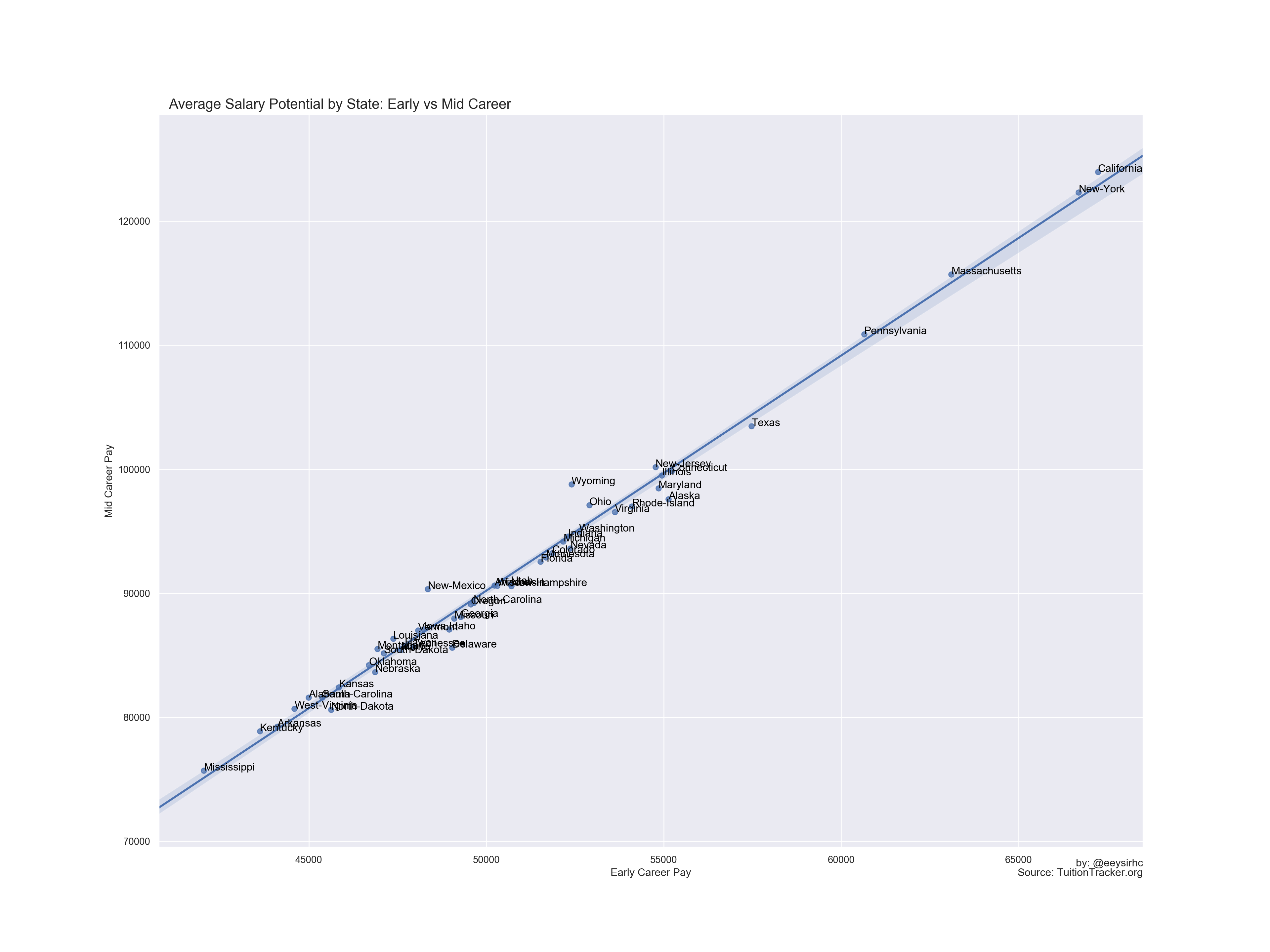
Now, all that is left is to find something catchy for the other days of the week - lol.