We may be inundated with data but sometimes collecting it can be a challenge in and of itself. A few reasons off the top of my head:
- Sparsity
- Difficult to measure
- Impractical to devote company resources to it
- Lack of technical expertise to actually build or acquire it
- Lazy (yours truly - except for that one time)
Through simulation we can generate our own dataset with the added benefit of fully understanding what features we choose to put in our models (or leave out).
In fact, a few of the machine learning models I wrote and put into production at work are based on simulated data!
This article will provide a quick walkthrough in getting you up and running using #rstats.
Background
I am in the market for a smart camera so while shopping online I also compiled some page speed data for a few eCommerce websites. You can follow along with the data here:
library(tidyverse)
library(scales)
library(knitr)
library(kableExtra)

df <- read_csv("https://raw.githubusercontent.com/Eeysirhc/random_datasets/master/page_speed_benchmark.csv")

# VIEW RANDOM SAMPLE
df_sample <- df %>%
sample_n(10) | website | page_type | product | time_to_interactive |
|---|---|---|---|
| Smarthome | Category | Electrical | 9.8 |
| Home Depot | Category | Sensors | 25.1 |
| IKEA | Category | Entertainment | 9.8 |
| Smarthome | Category | Sensors | 9.8 |
| Smarthome | Category | Electrical | 8.9 |
| Amazon | Category | Sensors | 7.1 |
| Walmart | Category | Sensors | 15.9 |
| Amazon | Home |
|
10.4 |
| Amazon | Category | Sensors | 7.1 |
| BestBuy | Category | Sensors | 29.4 |
I used Google Chrome’s built-in page audit (Lighthouse) to log the time for each website, page type and product category.
There are other page speed metrics but for educational purposes we’ll just focus on using time_to_interactive.
Lets pose the question: which site is fastest in terms of time_to_interactive?
Standard approach
One way to answer that question is to create descriptive statistics by computing the averages, finding the percent difference from the fastest site and then calling it a day.
df_standard <- df %>%
  filter(page_type != 'Home') %>%
  group_by(website) %>%
  summarize(time_interactive = mean(time_to_interactive)) %>%
  ungroup() %>%
  arrange(time_interactive) %>%
  mutate(slower_than_amazon = round((time_interactive / 7.59 - 1) * 100, 0),
slower_than_amazon = paste0(slower_than_amazon, "%")) | website | time_interactive | slower_than_amazon |
|---|---|---|
| Amazon | 7.59000 | 0% |
| IKEA | 9.44000 | 24% |
| Smarthome | 9.44375 | 24% |
| Walmart | 16.63077 | 119% |
| Target | 21.36667 | 182% |
| Home Depot | 25.20000 | 232% |
| BestBuy | 31.23077 | 311% |
However, there is a problem - sample size!
df_size <- df %>%
  filter(page_type != 'Home') %>%
  group_by(website) %>%
  summarize(time_interactive = mean(time_to_interactive),
            count = n()) %>%
  ungroup() %>%
arrange(desc(count))| website | time_interactive | count |
|---|---|---|
| Smarthome | 9.44375 | 16 |
| BestBuy | 31.23077 | 13 |
| Walmart | 16.63077 | 13 |
| Amazon | 7.59000 | 10 |
| Home Depot | 25.20000 | 10 |
| Target | 21.36667 | 6 |
| IKEA | 9.44000 | 5 |
eCommerce sites have hundreds of thousands of pages so how can we be so certain our summary captures actual page speed performance? Perhaps adding in a confidence interval?
At a more granular level, IKEA and Smarthome have exactly the same average time_to_interactive of 9.44 seconds but I recorded fewer samples with the former - which site is actually faster?
df %>%
  filter(website %in% c('IKEA', 'Smarthome')) %>%
  ggplot(aes(website, time_to_interactive, color = website)) +
  geom_point(show.legend = FALSE, size = 5, alpha = 0.5) +
  geom_hline(yintercept = 9.44, lty = 2, color = 'red') +
  scale_color_manual(values = cbPalette3) +
  scale_y_continuous(limits = c(0, 15)) +
  labs(x = NULL, y = "Time to Interactive (seconds)",
       subtitle = "Dashed line represents average of 9.44s")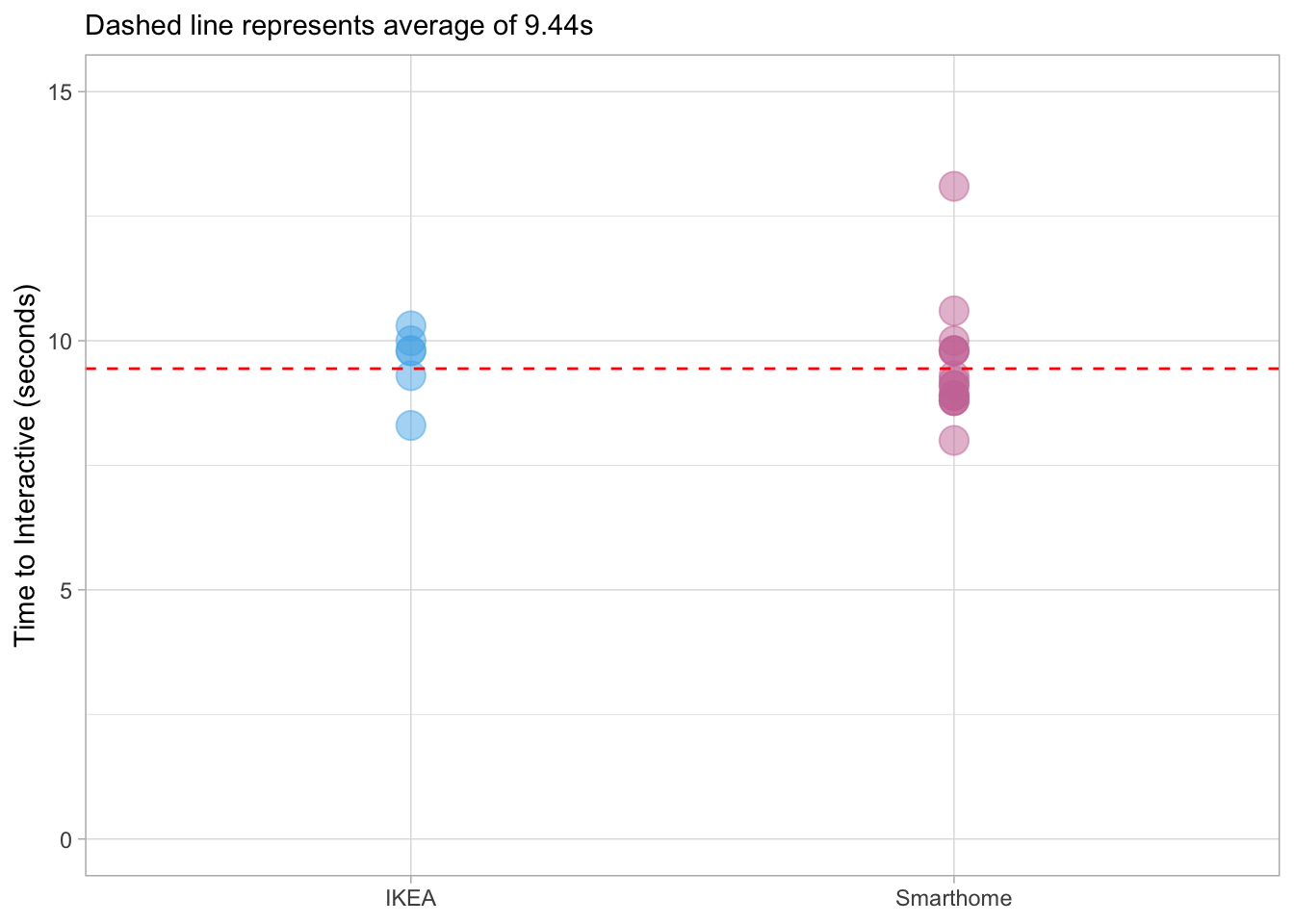
What if I don’t know how to write a script to grab every URL and then feed it into Google Lighthouse? Or more realistically, what if I am not inclined to go and collect 11 more data points for IKEA?
These questions can be answered with the help of simulation. By applying the central limit theorem and law of large numbers we can directly address measurement uncertainty.
Simulating “big” data
To get started we will need three values:
- n = number of observations
- mean = vector of means
- sd = vector of standard deviations
df_summary <- df %>%
  filter(page_type != 'Home') %>%
  group_by(website) %>%
  summarize(time_interactive = mean(time_to_interactive),
            sd = sd(time_to_interactive),
            count = n()) %>%
  ungroup() %>%
arrange(time_interactive)| website | time_interactive | sd | count |
|---|---|---|---|
| Amazon | 7.59000 | 1.9081405 | 10 |
| IKEA | 9.44000 | 0.6877500 | 5 |
| Smarthome | 9.44375 | 1.1488944 | 16 |
| Walmart | 16.63077 | 0.8300448 | 13 |
| Target | 21.36667 | 2.0175893 | 6 |
| Home Depot | 25.20000 | 1.4055446 | 10 |
| BestBuy | 31.23077 | 2.6042864 | 13 |
Now that we have the minimum requirements we can simulate our data. Let’s start with IKEA:
ikea <- rnorm(1e4, 9.44, 0.688) %>%
  as_tibble() %>%
  mutate(website = paste0("ikea"))
There was a lot to unpack there so let’s break it down:
- rnorm is the R function to generate random numbers from a Gaussian distribution
- 1e4 is scientific notation for 10,000 observations
- 9.44 is the average mean for IKEA time_to_interactive
- 0.688 is the standard deviation
- We moved our data into the tidyverse with as_tibble()
- Used the mutate function to add a website column and identify IKEA for the set of results
We can now plot our distribution of time_to_interactive scores for IKEA where we generated 10K data points.
ikea %>%
  ggplot(aes(value, fill = website)) +
  geom_histogram(position = 'identity', binwidth = 0.05, alpha = 0.8,
                 show.legend = FALSE) +
  scale_fill_manual(values = cbPalette) +
  scale_x_continuous(limits = c(0, 20)) +
  labs(x = "Time to Interactive (seconds)", y = NULL)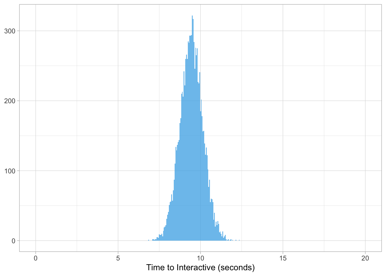
What this illustrates is the potential frequency of page speed scores and the range of all possible values.
In other words, if we take a random page on IKEA and measure its time_to_interactive we know scores could be as low as 8s or as high as 11s. Additionally, there is a central tendency for scores to fall around 9s but it is not at all possible to have a score of 1s or more than 13s.
This is an improvement from a single summary statistic but what if we wanted to ask more complicated questions? What if we wanted to know the likelihood a random IKEA page was greater than 11s? Or which site is faster: Amazon vs IKEA?
The solution is to condition on our simulated dataset.
Conditioning on the imaginary
Lets ask the question: what is the probability IKEA will have a page speed greater than 11 seconds?
We can easily get that answer by sampling from our data:
sum(ikea$value > 11) / length(ikea$value) * 100## [1] 1.45And to drive that home with some data viz…
ikea %>%
  mutate(greater_11s = ifelse(value > 11, 'yes', 'no')) %>%
  ggplot(aes(value, fill = greater_11s)) +
  geom_histogram(binwidth = 0.05, alpha = 0.7) +
  scale_fill_manual(values = cbPalette) +
  scale_x_continuous(limits = c(0, 20)) +
labs(x = "Time to Interactive (seconds)", y = NULL) 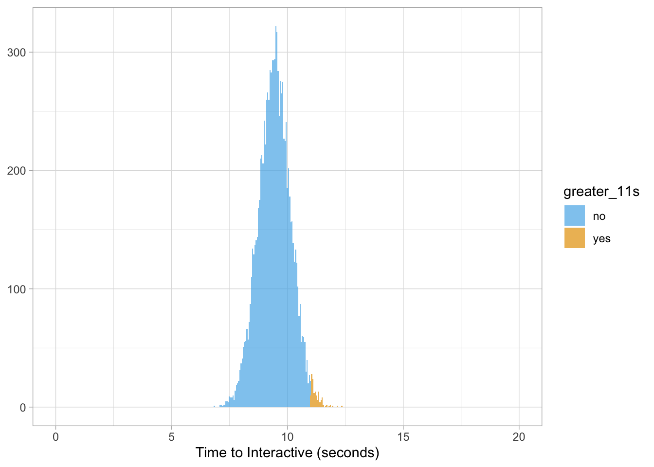
We can also head in the opposite direction: what is the probability IKEA will have a page speed of less than 9 seconds?
sum(ikea$value < 9) /length(ikea$value) * 100## [1] 25.72And to plot our results…
ikea %>%
  mutate(less_than_9s = ifelse(value < 9, 'yes', 'no')) %>%
  ggplot(aes(value, fill = less_than_9s)) +
  geom_histogram(binwidth = 0.05, alpha = 0.7) +
  scale_fill_manual(values = cbPalette) +
  scale_x_continuous(limits = c(0, 20)) +
labs(x = "Time to Interactive (seconds)", y = NULL) 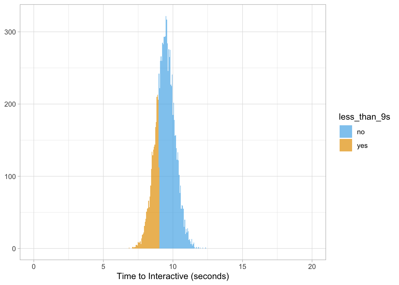
We can also ask more complicated quesitons such as: what is the probability a random Amazon page will be faster than IKEA?
# SIMULATE AMAZON DATA
amazon <- rnorm(1e4, 7.59, 1.91) %>%
  as_tibble() %>%
  mutate(website = paste0("amazon"))

mean(amazon$value < ikea$value) * 100
## [1] 82.39And…well…you get the idea….
pagespeed <- rbind(ikea, amazon)

pagespeed %>%
  ggplot(aes(value, fill = website)) +
  geom_histogram(binwidth = 0.05, alpha = 0.7, position = 'identity') +
  scale_fill_manual(values = cbPalette2) +
  scale_x_continuous(limits = c(0, 20)) +
labs(x = "Time to Interactive (seconds)", y = NULL) 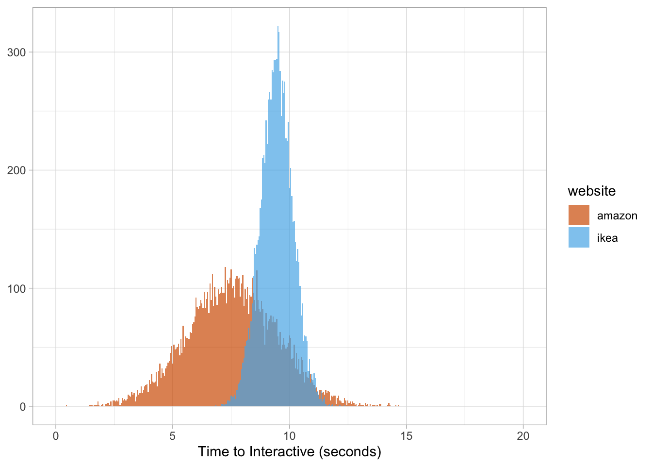
Side note
From my personal experience working at large companies, business executives respond very well to probabilities. Thus, “our site is 24% slower than Amazon” is not as impactful as stating “if we were to take 10K random pages from each site, there is an 82% chance our site will be slower than Amazon.”
What about Amazon?
In the past I wrote about segmenting data to reveal deeper insights hidden beneath the aggregation.
So, what is really driving Amazon’s page speed score higher? Lets simulate some data and for fun we’ll increase our observations from 1e4 (10K) to 1e5 (100K). Quick reminder about Amazon page speed data:
df_amazon <- df %>%
  filter(website == 'Amazon', page_type != 'Home') %>%
  group_by(product) %>%
  summarize(time_interactive = mean(time_to_interactive),
            sd = sd(time_to_interactive)) %>%
arrange(time_interactive)| product | time_interactive | sd |
|---|---|---|
| Electrical | 5.750000 | 0.212132 |
| Security | 7.933333 | 2.458319 |
| Sensors | 8.066667 | 1.674316 |
| Entertainment | 8.200000 | 2.545584 |
And the code to generate our data with the subsequent plot:
electrical <- rnorm(1e5, 5.75, 0.212) %>% as_tibble() %>%
  mutate(product = paste0("electrical"))

security <- rnorm(1e5, 7.93, 2.46) %>% as_tibble() %>%
  mutate(product = paste0("security"))

sensors <- rnorm(1e5, 8.07, 1.67) %>% as_tibble() %>%
  mutate(product = paste0("sensors"))

entertainment <- rnorm(1e5, 8.2, 2.55) %>% as_tibble() %>%
  mutate(product = paste0("entertainment"))

amazon <- rbind(electrical, security, sensors, entertainment)

amazon %>%
  ggplot(aes(value, fill = product)) +
  geom_histogram(binwidth = 0.05, alpha = 0.7, position = 'identity') +
  scale_x_continuous(limits = c(0, 20)) +
  scale_y_continuous(labels = comma_format()) +
  scale_fill_brewer(palette = 'Spectral') +
  labs(x = "Time to Interactive (seconds)", y = NULL,
       title = "Amazon: time to interactive by product category (n=100K)")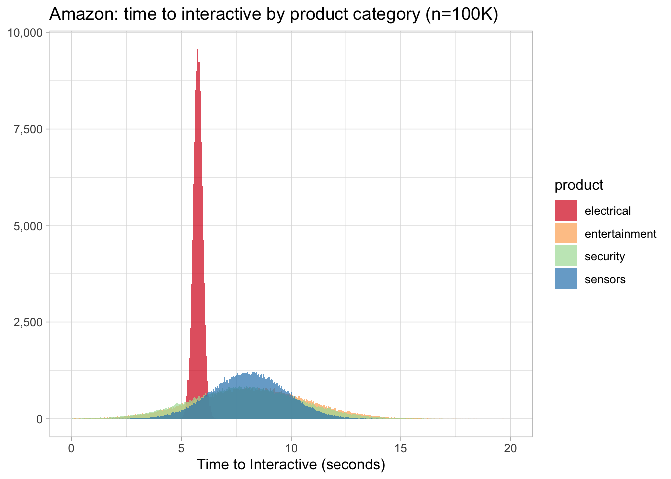
Well, this is quite shocking (pun intended) - the electrical category’s time_to_interactive is not only faster but its central tendency is also less dispersed than the other three.
Why might that be the case? Specific business focus on these products? Less teams working on it? Not enough products? All conjecture on my part without digging deeper into the site.
Finally, what is the probability the electrical category is faster than security (2nd place)?
mean(electrical$value < security$value) * 100## [1] 81.145Wrapping up
With data simulation we can account for sample size, uncertainty and interpretability. We can achieve this understanding without building something entirely new either.
This methodology can be applied to any aspect of digital marketing where data is the lifeblood of the channel. For example…
- Rankings: your daily rank went from #9 to #1 only to celebrate too early and it drops back down to #8 the next day. If you calculated the probability of hitting #1 from the source data, would you not have celebrated as early?
- Traffic: was the spike in site visitors a real phenomenon or just random chance?
- Click-through Rate: how do you handle low volume data where you only received 2 clicks and 2 impressions? You don’t want to kick out data because it is telling you something! (check out my R guide and the section on estimating CTR with empirical Bayes)
Intentional exclusion
I specifically left out certain concepts to get the reader excited about using R to simulate their own data. Although important, I will leave those for future articles but the following are notes for myself:
- Foundation for Bayesian statistics
- No mention of incorporating conjugate priors
- Other R distribution functions: dnorm, pnorm, qnorm
- Minimized mathematical notation