One of my dogs was recently diagnosed with an enlarged heart so the vet prescribed some medicine to mitigate the problem. The box came with a pamphlet which included the company’s effectiveness study for the drug, Vetmedin.
I thought it would be fun to visualize one portion of the study with simulation. What follows is the #rstats code I used to examine and review the drug’s efficacy based on the reported results.
Load libraries
library(tidyverse)
library(scales)
Encode data
For this post we’ll focus only on the Treatment Success on Day 29 section.
Vetmedin Group (experiment)
- n = 134
- Success rate = 80.7%
exp_success <- 134 * 0.807
exp_failure <- 134 - exp_success
Active Control Group
- n = 131
- Success rate = 76.3%
ctl_success <- 131 * 0.763
ctl_failure <- 131 - ctl_success
Create simulation function
We’ll simulate 10K trials for each group (total of 20K) using the beta distribution since it is easier to work with when the data is framed as “successful” vs “not successful”.
med_sim <- function(x, y, segment){
  values <- rbeta(1e4, x, y) %>%
    as_tibble() %>%
    mutate(segment = paste0(segment))
}
Simulate survey data
exp <- med_sim(exp_success, exp_failure, "experiment")
ctl <- med_sim(ctl_success, ctl_failure, "control")
Is the experiment better than the control group?
exp_sig <- mean(exp$value > ctl$value) * 100

bind_rows(exp, ctl) %>%
  ggplot(aes(value, fill = segment)) +
  geom_histogram(binwidth = 0.005, alpha = 0.8, position = 'identity') +
  scale_x_continuous(labels = percent_format(round(1))) +
  scale_fill_brewer(palette = 'Set1') +
  labs(title = "Vetmedin: effectiveness results for the 29-day field study",
       subtitle = paste0(exp_sig, "% chance experiment is greater than control (MC sampling of 10K per group)"),
       caption = "by: @eeysirhc\nsource: FDA (NADA 141-273)",
       x = "Success Rate on Day 29",
       y = NULL,
       fill = NULL) +
  theme_minimal() +
  theme(axis.text.y = element_blank(),
        axis.ticks.y = element_blank(),
legend.position = 'top') 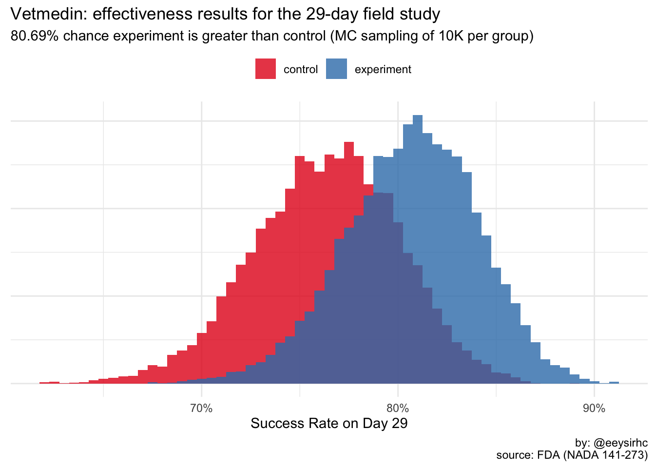
Interesting - it looks like the statistical significance threshold for this canine medication was set at 80%.
I wonder if drugs for humans have the same or different minimum?
How much better is the experiment over control?
Knowing if we achieved statistical significance is good but it would be better if we knew by how much.
avg_improvement <- median(exp$value / ctl$value - 1)

improvement <- as_tibble((exp$value / ctl$value) - 1) %>%
  mutate(segment = ifelse(value > 0.00, 'experiment', 'control'))

improvement %>%
  ggplot(aes(value, fill = segment)) +
  geom_histogram(binwidth = 0.005, alpha = 0.8) +
  geom_vline(xintercept = avg_improvement, lty = 2, color = 'red') +
  scale_x_continuous(labels = percent_format(round(1))) +
  scale_y_continuous(labels = comma_format()) +
  scale_fill_brewer(palette = 'Set1') +
  labs(y = "Frequency",
       x = NULL,
       fill = NULL,
       title = "Vetmedin: effectiveness results for the 29-day field study",
       subtitle = paste0("Estimated ", round((avg_improvement * 100), 2), "% improvement of experiment over control (", exp_sig, "% significance)"),
       caption = "by: @eeysirhc\nsource: FDA (NADA 141-273)") +
  theme_minimal() +
theme(legend.position = 'top') 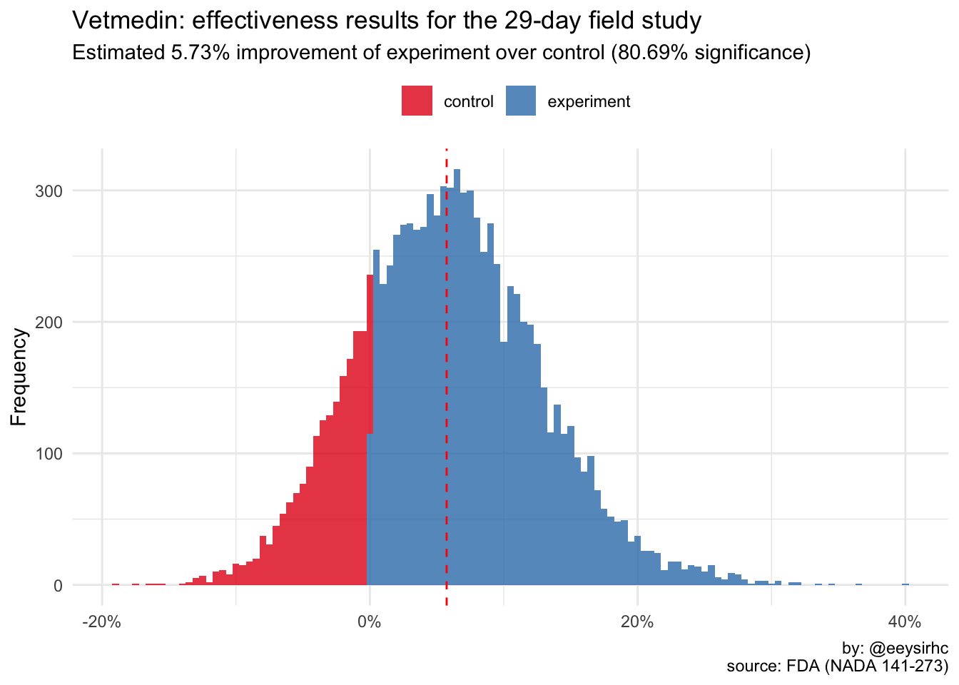
Thus, the Vetmedin study observed an average of +6% improvement over the control group at ~81% significance.
Since we simulated a total dataset of 20K trials we actually see a range of potential values from the low end of +1% to the extremes of over +20%. Additionally, this illustrates there could be instances where the control group is better than the experiment.
Would you use it for your dog? That ultimately depends on how much risk you are willing to accept.
Wrapping up
For the uninitiated, this is one way to conduct A/B testing using Bayesian statistics. With the computational power we have on our computers it is no longer necessary to make silly statements such as “we need [insert arbitrary number] conversions to achieve statistical significance.”