Purchasing a car is a significant time and financial commitment.
There is so much at stake that the required song and dance with the sales manager don’t alleviate any fears about over paying. Thus, it is difficult to determine the equilibirum point at which the dealer will accept your offer versus how much you are willing to pay.
I decided to write this for a few reasons:
- I am in the market for a new car
- Rather than doing actual car shopping I thought it would be more fun to procrastinate
- Online calculators are quite clunky when you want to compare and contrast monthly payments
- Hopefully, this will help others make more informed car buying decisions (TBD on Shiny app)
Note: this guide will focus only on leasing and not the auto financing aspect of it
Lease payment calculations
Our variables are split in two categories:
- What you know
- MSRP (or sticker price)
- Lease term (months)
- Down payment
- Local sales tax
- What the dealer knows
- Sales price (how much they will discount off MSRP)
- Residual
- Money factor (or APR)
- Rebates, incentives and credits
- Fees
- Trade-in value
re: money factor & APR
To find the money factor from APR divide by 2,400
To find the APR from money factor multiply by 2,400
Here is the formula to calculate our monthly lease payments:
monthly_payment = [depreciation_fee + finance_fee] * sales_tax
However, to plug in those numbers a lot of math has to happen beforehand but you can read the full definitions here on Edmunds.
We’ll lay them all out below for reference:
capitalized_costs = [sales_price + fees] - down_payment - trade_in - rebate
residual_value = msrp * residual
depreciation_fee = [capitalized_costs - residual_value] / lease_term
finance_fee = [capitalized_costs + residual_value] * money_factor
With the formalities out of the way we can now get to coding up our solution in #rstats.
Load packages
library(tidyverse)
library(scales)
Creating our function
R will do the heavy lifting for us and since we wrote down the entire formula it will be easy to build that function.
lease_calculation <- function(msrp, sales_price, residual, money_factor, rebate,
                              fees, term, down_payment, trade_in, tax){
  # CAPITALIZED COSTS
  capcosts <- (sales_price + fees) - down_payment - trade_in - rebate

  # RESIDUAL VALUE
  residual_value <- msrp * residual

  # DEPRECIATION FEE
  depreciation_fee <- (capcosts - residual_value) / term

  # FINANCE FEE
  finance_fee <- (capcosts + residual_value) * money_factor

  # TOTAL MONTHLY PAYMENT
  monthly_payment <- (depreciation_fee + finance_fee) * (1 + (tax / 100))

  # ROUND TO TWO DECIMAL PLACES
  round(monthly_payment, 2)
}
Now we can plug in the values from the Edmunds example:
payment <- lease_calculation(msrp = 23000,
                  sales_price = 21000,
                  residual = 0.57,
                  money_factor = 0.00125,
                  rebate = 500,
                  fees = 1200,
                  term = 36,
                  down_payment = 1700,
                  trade_in = 0,
                  tax = 10.25)

cat(paste0("Monthly lease payment: $", payment))
## Monthly lease payment: $256.64Awesome - this is working as intended!
Note: if you are lucky enough to not live in a state requires rolling the sales taxes into your monthly payment then feel free to set tax=0
Comparing offers
Single point estimates are great but we may want to simulate multiple lease offers so we know what negotation levers are at our disposal to stay within budget.
lease_comparison <- function(msrp, sales_price, residual, money_factor, rebate,
                             fees, term, down_payment, trade_in, tax){

  capcosts <- (sales_price + fees) - down_payment - trade_in - rebate
  residual_value <- msrp * residual
  depreciation_fee <- (capcosts - residual_value) / term
  finance_fee <- (capcosts + residual_value) * money_factor
  sales_tax <- (depreciation_fee + finance_fee) * tax
  monthly_payment <- (depreciation_fee + finance_fee) * (1 + (tax / 100))

  # NEW CODE: JOIN SALES PRICE AND MONTHLY PAYMENT
  as_tibble(cbind(sales_price, monthly_payment))
}
Let’s use our updated lease_comparison function and assume we are looking to lease a brand new BMW M4.
A fully loaded one has an MSRP of about $85,000, residual is typically 60%, APR in January 2020 was about 3.288%, dealers typically throw in a few hundred dollars to ease the pain and the sales tax where I live is 9.5%.
We’ll lay out three different scenarios where everything is equal with the exception of our down payment.
down5k <- lease_comparison(msrp = 85000,
                  sales_price = 78200, # 8% DISCOUNT OFF STICKER
                  residual = 0.60,
                  money_factor = 0.00137,
                  rebate = 500,
                  fees = 0,
                  term = 36,
                  down_payment = 5000,
                  trade_in = 0,
                  tax = 9.5) %>%
  mutate(offer = '5k_down_payment')

down2k <- lease_comparison(msrp = 85000,
                  sales_price = 78200,
                  residual = 0.60,
                  money_factor = 0.00137,
                  rebate = 500,
                  fees = 0,
                  term = 36,
                  down_payment = 2000,
                  trade_in = 0,
                  tax = 9.5) %>%
  mutate(offer = '2k_down_payment')

down0 <- lease_comparison(msrp = 85000,
                  sales_price = 78200,
                  residual = 0.60,
                  money_factor = 0.00137,
                  rebate = 500,
                  fees = 0,
                  term = 36,
                  down_payment = 0,
                  trade_in = 0,
                  tax = 9.5) %>%
  mutate(offer = 'no_down_payment')

rbind(down5k, down2k, down0)
## # A tibble: 3 x 3
## sales_price monthly_payment offer
## <dbl> <dbl> <chr>
## 1 78200 846. 5k_down_payment
## 2 78200 941. 2k_down_payment
## 3 78200 1005. no_down_paymentAs expected a higher down payment leads to a lower monthly payment.
This is just OK and I think we can do better.
Visualizing uncertainty
Online car lease calculators only provide estimates and there will always be things we don’t know what we don’t know.
We might get an output of $900 but when we get to the sales floor the total monthly payment at signing could go up or down for a number of reasons.
To plan ahead, we can incorporate some of this uncertainty and visualize what the range of possible values might be given our inputs.
set.seed(20200312)

lease_rnorm <- function(n, price, offer){

  # ASSUME GAUSSIAN DISTRIBUTION
  rnorm(n, price, 6) %>% # ASSIGNED STANDARD DEVIATION OF 6
    as_tibble() %>%
    mutate(offer = offer)
}

# GENERATE 10K SAMPLES FOR EACH SCENARIO
down5k_sim <- lease_rnorm(1e4, down5k$monthly_payment, down5k$offer)
down2k_sim <- lease_rnorm(1e4, down2k$monthly_payment, down2k$offer)
down0_sim <- lease_rnorm(1e4, down0$monthly_payment, down0$offer)

# COMBINE DATA FRAMES
final_sim <- rbind(down5k_sim, down2k_sim, down0_sim)

# PLOT CHART
final_sim %>%
  ggplot(aes(value, fill = offer)) +
  geom_histogram(alpha = 0.8, binwidth = 0.5) +
  scale_x_continuous(labels = dollar_format(),
                     limits = c(800, 1100)) +
  labs(y = NULL, x = "monthly_payment") +
  facet_grid(offer ~ .) +
  theme_bw() +
  theme(legend.position = 'none',
        axis.text.y = element_blank())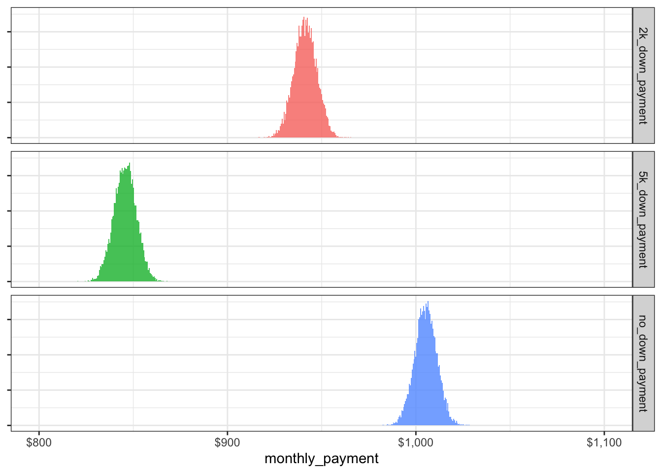
So, what are we looking at? We’ll zoom in on the no_down_payment option:
summary(down0_sim)## value offer
## Min. : 982.7 Length:10000
## 1st Qu.:1001.3 Class :character
## Median :1005.3 Mode :character
## Mean :1005.2
## 3rd Qu.:1009.2
## Max. :1028.5We know the calculator returned a monthly payment of $1,005. However, when we include some uncertainty in our estimate we can expect a minimum of $983 to a maximum monthly payment of $1,039.
Extracting probabilities
Since we now know the range of possible monthly payment values, we can also use it to figure out the probability of negotiating for a lower price.
The plot below illustrates the probability distribution of monthly lease payments for our 2k_down_payment option:
ggplot(data.frame(x = c(800, 1100)), aes(x)) +
  stat_function(args = c(mean = mean(down2k_sim$value), sd = 6),
                aes(color = 'steelblue'),
                fun = pnorm,
                n = 1e4,
                size = 1) +
  geom_vline(xintercept = mean(down2k_sim$value), lty = 2) + # ESTIMATED MONTHLY
  theme_bw() +
  scale_x_continuous(labels = dollar_format()) +
  scale_y_continuous(labels = percent_format()) +
  labs(x = NULL, y = NULL)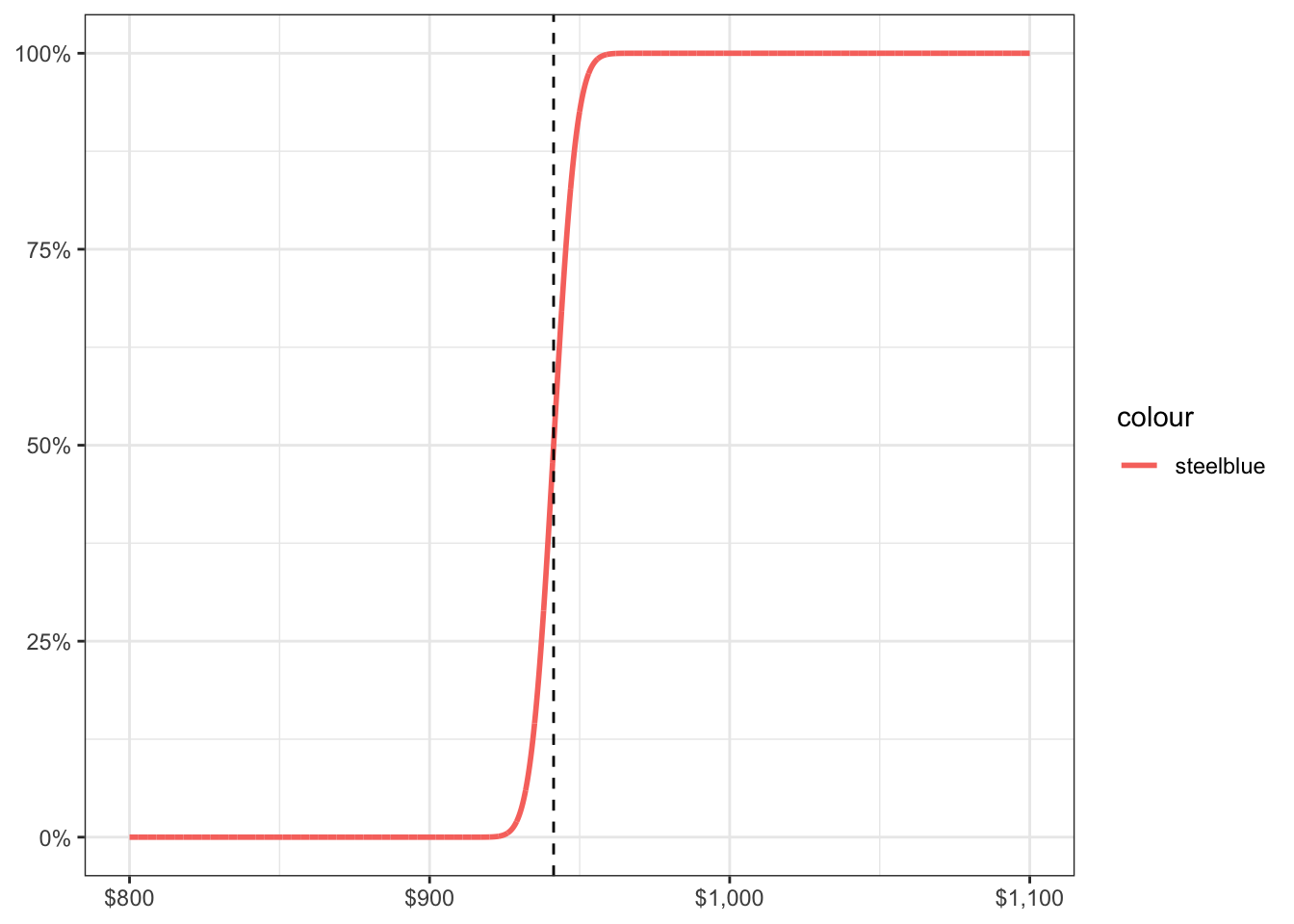
The estimated monthly payment is $941 which coincides with a 50% chance we will actually receive that offer from the dealership.
We should always be aggressive in these negotations so let’s figure out: what is the maximum monthly payment if I want to walk away with a 20% chance of getting the deal that I want?
qnorm(.20, mean(down2k_sim$value), 6)## [1] 936.2743At $936 that is about $180 saved over the course of the 3-year lease - not bad and in my opinion it’s worth asking for it.
If we are on a tight budget and can only do $930 per month then we can easily calculate those probabilities:
pnorm(930, mean(down2k_sim$value), 6) * 100## [1] 2.955695What this means is based on the values we set earlier ($2k down payment, 8% off sticker, etc.) there is a ~3% chance we’ll be able to walk away with a monthly payment of $930 instead of the original estimate of $941.
Wrapping up
We learned how the payments are calculated, the levers at our disposal to influence the monthly lease payment as well as compare and visualize multiple offers.
Shopping for a car can be stressful but I hope this guide on using R can calm down any jitters you may have for a future decision.
Resources
If you enjoyed this article, you may like a few other guides I wrote in the past: